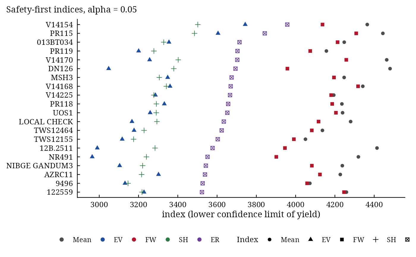
stab_eskridge() computes the four safety-first selection indices of Eskridge (1990). Each index is a lower
confidence limit of a genotype's yield: the mean minus a multiple of a stability measure. The breeder who wants a
small probability alpha of a disastrously low yield prefers the genotype with the largest index (Kataoka's
safety-first rule). The indices weigh yield against stability explicitly through alpha.
Usage
stab_eskridge(.data, .y, .rep, .gen, .env, alpha = 0.05)

# Default S3 method
stab_eskridge(.data, .y, .rep, .gen, .env, alpha = 0.05)
Arguments
- .data
a data frame (or
data.table) with one row per plot.- .y
response: a column of
.datagiven by name (.y = Yieldor.y = "Yield") or a numeric vector of lengthnrow(.data).- .rep
replicate: not used (kept for compatibility); may be omitted.
- .gen
genotype: a column of
.dataor a vector, as for.y.- .env
environment: a column of
.dataor a vector, as for.y.- alpha
probability of a disastrously low yield that the breeder accepts (default
0.05).
Value
An object of class c("stab_eskridge", "stab_result", "list"):
Eskridgedata.tablesorted byER:Gen,Mean,EV,FW,SH,ERand their ranksrMean,rEV,rFW,rSH,rER(1 = largest).Parametersdata.table:Gen,Mean,S2(variance over environments),b(slope),Sigma2(Shukla's variance),S2d(deviation mean square).Constantsnamed vector:
z,S2y,Sigma2E,alpha.RankCormatrix of Kendall's rank correlations between the mean and the four indices (Eskridge's Table 5).
Methods: print(), summary(), plot() (which = c("indices", "ranks")),
stab_interpret().
Details
With \(Z = Z_{1-\alpha}\), the \(1 - \alpha\) quantile of the standard normal distribution, the table of means \(\bar{y}_{ij}\) of \(G\) genotypes in \(E\) environments and the environment index \(I_j = \bar{y}_{\cdot j} - \bar{y}\): $$EV_i = \bar{y}_{i\cdot} - Z\,S_i, \qquad FW_i = \bar{y}_{i\cdot} - Z\left[(b_i - 1)^2 S_y^2 (1 - 1/E) \right]^{1/2},$$ $$SH_i = \bar{y}_{i\cdot} - Z\left[\hat{\sigma}^2_E + \hat{\sigma}^2_i\right]^{1/2}, \qquad ER_i = \bar{y}_{i\cdot} - Z\left[(b_i - 1)^2 S_y^2 (1 - 1/E) + S^2_{d_i}\right]^{1/2},$$ where \(S^2_i = \sum_j(\bar{y}_{ij} - \bar{y}_{i\cdot})^2/(E - 1)\) is the variance over environments, \(b_i = \sum_j(\bar{y}_{ij} - \bar{y}_{i\cdot})I_j/\sum_j I_j^2\) Finlay and Wilkinson's slope, \(S_y^2 = \sum_j I_j^2/(E - 1)\) the variance of the environment means, \(\hat{\sigma}^2_i\) Shukla's stability variance, \(\hat{\sigma}^2_E = [MS(E) - MS(GE)]/G\) the environmental variance component with \(MS(E) = G\sum_j I_j^2/(E - 1)\) and \(MS(GE) = \sum_{ij} z_{ij}^2/((G - 1)(E - 1))\), and \(S^2_{d_i} = [\sum_j(\bar{y}_{ij} - \bar{y}_{i\cdot})^2 - b_i^2 \sum_j I_j^2]/(E - 2)\) the mean square of the deviations from regression (Eskridge 1990, Table 1).
The four indices rest on four definitions of stability (Lin et al. 1986): EV on the variance over environments
(type 1), FW and SH on the response relative to the other genotypes (type 2), ER on type 2 and the unpredictable
deviations (type 3). EV favours genotypes that vary little, whatever the environments; FW, SH and ER favour
genotypes that follow the average response. Small alpha weighs stability heavily (a breeder or farmer who
cannot afford a poor yield); alpha near 0.5 (\(Z = 0\)) reduces every index to the mean.
Eskridge used \(\alpha = 0.05\) and notes that subsistence farmers have shown \(Z\) between 0.5
and 1.5 (\(\alpha\) between 0.30 and 0.05).
References
Eskridge, K. M. (1990). Selection of stable cultivars using a safety-first rule. Crop Science, 30(2), 369–374.
Kataoka, S. (1963). A stochastic programming model. Econometrica, 31(1–2), 181–196.
Lin, C. S., Binns, M. R. and Lefkovitch, L. P. (1986). Stability analysis: where do we stand? Crop Science, 26(5), 894–900.
See also
stab_reliability, stab_measures, stab_interpret
Other stability analyses:
add_anova(),
ammi(),
ammi_biplot(),
er_anova(),
ge_effects(),
ge_means(),
gge_biplot(),
indiv_anova(),
stab_asv(),
stab_dist(),
stab_fox(),
stab_huehn(),
stab_kang(),
stab_masv(),
stab_measures(),
stab_par(),
stab_reg(),
stab_reliability(),
stab_superiority()
Author
Muhammad Yaseen (myaseen208@gmail.com), Kent M. Eskridge (keskridge1@unl.edu)
Examples
data(ge_data)
fit <-
  stab_eskridge(
      .data = ge_data
    , .y    = Yield
    , .rep  = Rep
    , .gen  = Gen
    , .env  = Env
    , alpha = 0.05
    )
head(fit$Eskridge)
#>         Gen     Mean       EV       FW       SH       ER rMean   rEV   rFW
#>      <char>    <num>    <num>    <num>    <num>    <num> <int> <int> <int>
#> 1:   V14154 4364.727 3743.343 4136.892 3501.802 3957.406     5     1    11
#> 2:    PR115 4444.273 3604.917 4308.500 3485.151 3842.936     3     2     2
#> 3: 013BT034 4247.500 3355.062 4213.649 3328.587 3714.264    11     5     5
#> 4:    PR119 4156.727 3200.607 4074.380 3278.279 3703.990    24    16    16
#> 5:   V14170 4463.818 3256.493 4258.024 3402.104 3702.917     2    13     3
#> 6:    DN126 4480.864 3047.967 3958.065 3379.643 3693.828     1    29    23
#>      rSH   rER
#>    <int> <int>
#> 1:     1     1
#> 2:     2     2
#> 3:     6     3
#> 4:    12     4
#> 5:     3     5
#> 6:     4     6
fit$RankCor
#>           Mean        EV        FW        SH        ER
#> Mean 1.0000000 0.4757062 0.6305085 0.7615819 0.6542373
#> EV   0.4757062 1.0000000 0.4881356 0.5175141 0.5096045
#> FW   0.6305085 0.4881356 1.0000000 0.6723164 0.6169492
#> SH   0.7615819 0.5175141 0.6723164 1.0000000 0.8926554
#> ER   0.6542373 0.5096045 0.6169492 0.8926554 1.0000000
plot(x = fit, which = c("indices", "ranks")[1])