ammi() fits the AMMI model: additive genotype and environment effects plus a sum of multiplicative terms
for the interaction, found by the singular value decomposition of the table of interaction effects (Gauch 1992).
It gives the combined analysis of variance, the split of the interaction into principal components with Gollob's
(1968) \(F\) tests, and the genotype and environment scores.
Arguments
- .data
a data frame (or
data.table) with one row per plot.- .y
response: a column of
.datagiven by name (.y = Yieldor.y = "Yield") or a numeric vector of lengthnrow(.data).- .rep
replicate (block within environment): a column of
.dataor a vector, as for.y.- .gen
genotype: a column of
.dataor a vector, as for.y.- .env
environment: a column of
.dataor a vector, as for.y.
Value
An object of class c("stab_ammi", "stab_result", "list") with the components of earlier versions:
anovathe combined analysis of variance of
add_anova.pc_anovadata.table, one row per axis:PC,SingVal,Percent,AccumPerc,Df,SS,MeanSq,Fvalue,ProbF.gen_scores,env_scoresmatrices of genotype and environment scores (columns
PC1,PC2, ...).
and a new one:
ammi_modelthe model suggested by the tests, e.g.
"AMMI2".
Methods: print(), summary(), plot() (which = c("scree", "ammi1", "ammi2")),
stab_interpret().
Details
The model for the cell means is $$\bar{y}_{ij} = \mu + g_i + e_j + \sum_{n=1}^{N}\lambda_n\gamma_{in}\delta_{jn} + \rho_{ij},$$ where \(\lambda_n\) are the singular values of the interaction matrix \(\mathbf{Z} = (z_{ij})\), \(z_{ij} = \bar{y}_{ij} - \bar{y}_{i\cdot} - \bar{y}_{\cdot j} + \bar{y}\), and \(\gamma_{in}\), \(\delta_{jn}\) its singular vectors. Axis \(n\) has the sum of squares \(B\lambda_n^2\) on \(G + E - 1 - 2n\) degrees of freedom (Gollob 1968) and is tested against the pooled error. The scores are \(\gamma_{in}\sqrt{\lambda_n}\) for genotypes and \(\delta_{jn}\sqrt{\lambda_n}\) for environments, so that their products give the interaction. The number of significant axes (tested in order, at 0.05) suggests the model: AMMI0 (no axis), AMMI1, AMMI2, ....
Changes from the earlier version. The table pc_anova lists the \(\min(G, E) - 1\)
axes that exist (the earlier version added a row of zeros); the interaction is computed from the table of means
directly (no refitted aov()).
References
Gauch, H. G. (1992). Statistical Analysis of Regional Yield Trials: AMMI Analysis of Factorial Designs. Elsevier, Amsterdam.
Gollob, H. F. (1968). A statistical model which combines features of factor analytic and analysis of variance techniques. Psychometrika, 33(1), 73–115. doi:10.1007/BF02289676
Zobel, R. W., Wright, M. J. and Gauch, H. G. (1988). Statistical analysis of a yield trial. Agronomy Journal, 80(3), 388–393. doi:10.2134/agronj1988.00021962008000030002x
See also
ammi_biplot, stab_asv, stab_masv, stab_dist,
stab_interpret
Other stability analyses:
add_anova(),
ammi_biplot(),
er_anova(),
ge_effects(),
ge_means(),
gge_biplot(),
indiv_anova(),
stab_asv(),
stab_dist(),
stab_eskridge(),
stab_fox(),
stab_huehn(),
stab_kang(),
stab_masv(),
stab_measures(),
stab_par(),
stab_reg(),
stab_reliability(),
stab_superiority()
Author
Muhammad Yaseen (myaseen208@gmail.com), Kent M. Eskridge (keskridge1@unl.edu)
Examples
data(ge_data)
fit <-
  ammi(
      .data = ge_data
    , .y    = Yield
    , .rep  = Rep
    , .gen  = Gen
    , .env  = Env
    )
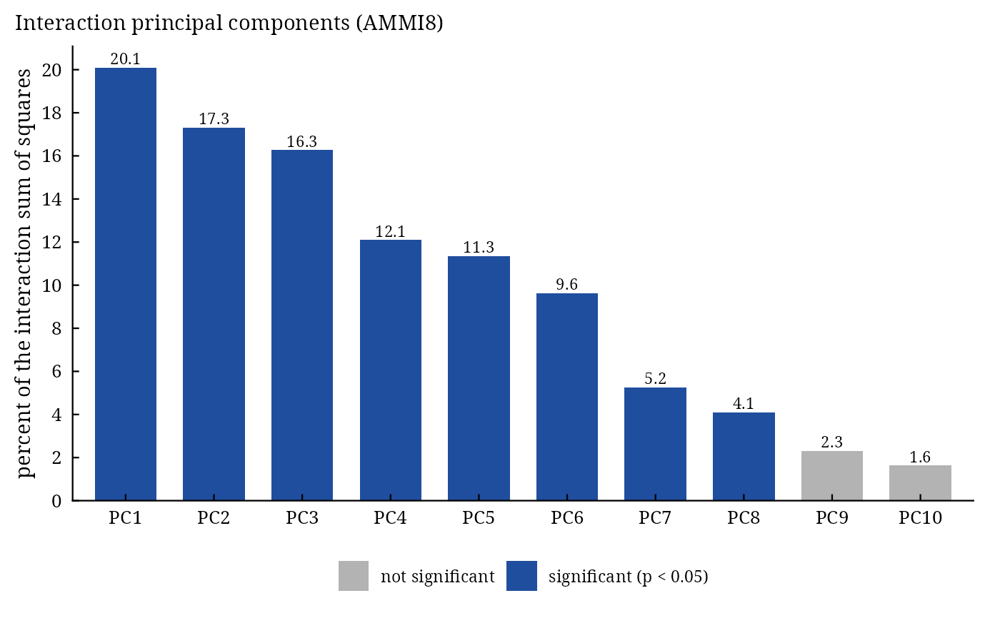
fit$pc_anova
#>         PC  SingVal   Percent AccumPerc    Df       SS    MeanSq    Fvalue
#>     <char>    <num>     <num>     <num> <num>    <num>     <num>     <num>
#>  1:    PC1 4496.142 20.081104  20.08110    68 40430588 594567.47 5.9956010
#>  2:    PC2 4174.531 17.311027  37.39213    66 34853411 528081.98 5.3251633
#>  3:    PC3 4046.566 16.266000  53.65813    64 32749392 511709.24 5.1600611
#>  4:    PC4 3489.555 12.096162  65.75429    62 24353985 392806.22 3.9610464
#>  5:    PC5 3380.195 11.349876  77.10417    60 22851440 380857.33 3.8405542
#>  6:    PC6 3113.224  9.627826  86.73199    58 19384326 334212.52 3.3701893
#>  7:    PC7 2297.953  5.245534  91.97753    56 10561173 188592.38 1.9017601
#>  8:    PC8 2030.472  4.095450  96.07298    54  8245635 152696.94 1.5397915
#>  9:    PC9 1521.907  2.300825  98.37380    52  4632399  89084.60 0.8983265
#> 10:   PC10 1279.478  1.626196 100.00000    50  3274127  65482.53 0.6603240
#>            ProbF
#>            <num>
#>  1: 2.428622e-36
#>  2: 1.511108e-30
#>  3: 1.150112e-28
#>  4: 3.679112e-19
#>  5: 7.571781e-18
#>  6: 4.018722e-14
#>  7: 1.448407e-04
#>  8: 9.520167e-03
#>  9: 6.770319e-01
#> 10: 9.659157e-01
fit$ammi_model
#> [1] "AMMI8"
plot(x = fit, which = c("scree", "ammi1", "ammi2")[1])