er_anova() gives Eberhart and Russell's (1966) analysis of variance of a multi-environment trial, which
splits the environments and the genotype-by-environment interaction into a linear part (the regression of each
genotype on the environment index) and the deviations from regression, with a test of the deviations of every
genotype, together with the stability parameters of each genotype.
Usage
er_anova(.data, .y, .rep, .gen, .env)

# Default S3 method
er_anova(.data, .y, .rep, .gen, .env)
Arguments
- .data
a data frame (or
data.table) with one row per plot.- .y
response: a column of
.datagiven by name (.y = Yieldor.y = "Yield") or a numeric vector of lengthnrow(.data).- .rep
replicate (block within environment): a column of
.dataor a vector, as for.y.- .gen
genotype: a column of
.dataor a vector, as for.y.- .env
environment: a column of
.dataor a vector, as for.y.
Value
An object of class c("stab_er_anova", "stab_result", "list") with the components of earlier
versions:
add_anovathe combined analysis of variance of
add_anova.er_anovaEberhart and Russell's analysis of variance (class
anova): linesTotal,Gen,Env + (Gen x Env),Env (linear),Gen x Env(linear),Pooled deviation, one line per genotype,Pooled error.
and a new one:
Parametersdata.table, one row per genotype:Gen,Mean,Slope(\(\hat{\beta}_i\)),SE,p.b1(test of \(\beta_i = 1\)),S2d(\(S^2_{d_i}\)),p.S2d(test of \(S^2_{d_i} = 0\)).
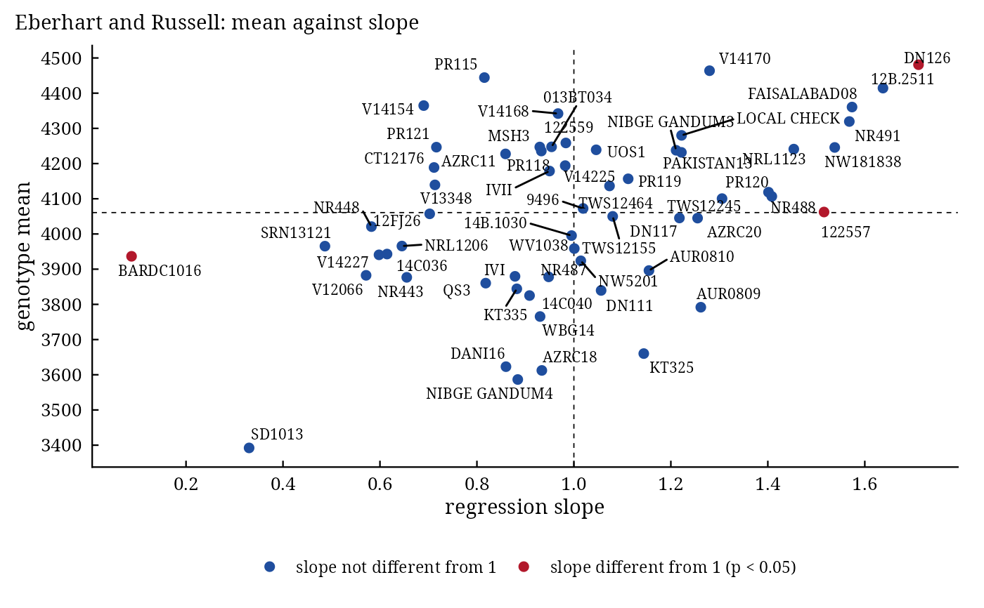
Methods: print(), summary(), plot() (mean against slope, which = "slope"; residuals,
which = "residuals" or "qq"), stab_interpret().
Details
With the table of means \(\mathbf{Y} = (\bar{y}_{ij})\) (\(G\) genotypes by \(E\) environments) and the environment index \(I_j = \bar{y}_{\cdot j} - \bar{y}\), every genotype is regressed on the index: $$\bar{y}_{ij} = \mu_i + \beta_i I_j + \delta_{ij}, \qquad \hat{\beta}_i = \frac{\sum_j \bar{y}_{ij}I_j}{\sum_j I_j^2}, \qquad S^2_{d_i} = \frac{\sum_j \hat{\delta}_{ij}^2}{E - 2} - \frac{s^2}{B},$$ where \(s^2\) is the pooled error mean square of the plots and \(B\) the number of replicates. On the scale of the means the analysis of variance is
| Total | \(GE - 1\) | \(\sum_{ij}(\bar{y}_{ij} - \bar{y})^2\) |
| Gen | \(G - 1\) | \(E\sum_i(\bar{y}_{i\cdot} - \bar{y})^2\) |
| Env + (Gen x Env) | \(G(E - 1)\) | \(\sum_{ij}(\bar{y}_{ij} - \bar{y}_{i\cdot})^2\) |
| Env (linear) | \(1\) | \(G\sum_j I_j^2\) |
| Gen x Env (linear) | \(G - 1\) | \(\sum_i(\sum_j\bar{y}_{ij}I_j)^2/\sum_j I_j^2 - G\sum_j I_j^2\) |
| Pooled deviation | \(G(E - 2)\) | \(\sum_{ij}\hat{\delta}_{ij}^2\) |
| Pooled error | \(f_e\) | \(f_e s^2/B\) |
Genotypes and the linear interaction are tested against the pooled deviation, the deviation of each genotype (\(E - 2\) degrees of freedom) against the pooled error. A stable genotype in the sense of Eberhart and Russell has a high mean, \(\beta_i = 1\) and \(S^2_{d_i} = 0\).
Changes from the earlier version. The lines Total and Gen used the replicate sum of squares; the deviation sums of squares were divided by the number of replicates (they are already on the scale of the means); the pooled error had \(EG(B - 1)\) instead of \(E(G - 1)(B - 1)\) degrees of freedom. All three are corrected, and the regression is computed in closed form (lme4 is no longer needed).
References
Eberhart, S. A. and Russell, W. A. (1966). Stability parameters for comparing varieties. Crop Science, 6(1), 36–40. doi:10.2135/cropsci1966.0011183X000600010011x
Singh, R. K. and Chaudhary, B. D. (2004). Biometrical Methods in Quantitative Genetic Analysis. Kalyani Publishers, New Delhi.
See also
stab_reg, add_anova, stab_interpret
Other stability analyses:
add_anova(),
ammi(),
ammi_biplot(),
ge_effects(),
ge_means(),
gge_biplot(),
indiv_anova(),
stab_asv(),
stab_dist(),
stab_eskridge(),
stab_fox(),
stab_huehn(),
stab_kang(),
stab_masv(),
stab_measures(),
stab_par(),
stab_reg(),
stab_reliability(),
stab_superiority()
Author
Muhammad Yaseen (myaseen208@gmail.com), Kent M. Eskridge (keskridge1@unl.edu)
Examples
data(ge_data)
fit <-
  er_anova(
      .data = ge_data
    , .y    = Yield
    , .rep  = Rep
    , .gen  = Gen
    , .env  = Env
    )
fit
#> Eberhart and Russell's analysis: 60 genotypes, 11 environments, 2 replicates
#>
#>                      Df    Sum Sq Mean Sq F value Pr(>F)
#> Total               659 268469701
#> Gen                  59  35831215  607309   3.777 <2e-16 ***
#> Env + (Gen x Env)   600 232638486
#>   Env (linear)        1 131970248
#>   Gen x Env(linear)  59  13847665  234706   1.460 0.0178 *
#>   Pooled deviation  540  86820573  160779
#> Pooled error        649  32179784   49584
#> ---
#> Signif. codes:  0 ‘***’ 0.001 ‘**’ 0.01 ‘*’ 0.05 ‘.’ 0.1 ‘ ’ 1
#>
#> (60 genotype deviation lines: x$er_anova; parameters: x$Parameters)
#>
#>              Gen  Mean  Slope     SE    p.b1    S2d     p.S2d
#>           <char> <num>  <num>  <num>   <num>  <num>     <num>
#>  1:        DN126  4481 1.7108 0.2412 0.01629  78341 6.340e-03
#>  2:       V14170  4464 1.2798 0.3003 0.37579 148757 5.436e-05
#>  3:        PR115  4444 0.8154 0.2401 0.46177  77256 6.794e-03
#>  4:     12B.2511  4414 1.6375 0.2844 0.05170 128304 2.261e-04
#>  5:       V14154  4365 0.6902 0.1384 0.05201  -7447 5.703e-01
#>  6: FAISALABAD08  4361 1.5737 0.3009 0.08897 149584 5.128e-05
#>  7:       V14168  4342 0.9673 0.2755 0.90807 117372 4.787e-04
#>  8:        NR491  4320 1.5681 0.2642 0.05997 103888 1.191e-03
#>  9:  LOCAL CHECK  4280 1.2221 0.2561 0.40827  94621 2.204e-03
#> 10:       122559  4259 0.9834 0.3015 0.95730 150380 4.849e-05
head(fit$Parameters)
#>         Gen     Mean     Slope        SE       p.b1       S2d        p.S2d
#>      <char>    <num>     <num>     <num>      <num>     <num>        <num>
#> 1: 013BT034 4247.500 0.9539767 0.2181489 0.83760871  55088.39 2.670478e-02
#> 2:   122557 4062.364 1.5159430 0.1702936 0.01425298  14201.74 2.406599e-01
#> 3:   122559 4258.591 0.9834026 0.3015181 0.95730445 150380.28 4.849012e-05
#> 4: 12B.2511 4414.409 1.6375025 0.2843871 0.05170192 128303.52 2.261371e-04
#> 5:   12FJ26 4057.227 0.7025845 0.2633342 0.28792236 102940.80 1.268556e-03
#> 6: 14B.1030 3995.409 0.9951608 0.2598803 0.98554993  98965.95 1.653205e-03
plot(x = fit, which = c("slope", "residuals", "qq")[1])