Stability parameters with Shukla's tests and Kang's yield-stability statistic

stab_par() gives Shukla's (1972) analysis of the genotype-by-environment interaction (its split into a heterogeneity part explained by an environmental covariate and a residual), the stability parameters of every genotype with $F$ tests of Shukla's stability variance, and Kang's (1993) yield-stability statistic $YS_i$ for selecting genotypes that are high-yielding and stable at the same time.

Usage

stab_par(.data, .y, .rep, .gen, .env, alpha = 0.1, .envCov = NULL)

# Default S3 method
stab_par(.data, .y, .rep, .gen, .env, alpha = 0.1, .envCov = NULL)

Arguments

.data: a data frame (or data.table) with one row per plot.
.y: response: a column of .data given by name (.y = Yield or .y = "Yield") or a numeric vector of length nrow(.data).
.rep: replicate (block within environment): a column of .data or a vector, as for .y.
.gen: genotype: a column of .data or a vector, as for .y.
.env: environment: a column of .data or a vector, as for .y.
alpha: level of the weakest significance that lowers the stability rating by 2 (default 0.1).
.envCov: environmental covariate: a column of .data (or a vector of length nrow(.data)) with one value per environment (rainfall, an index measured independently); NULL (default) uses the environment index.

Value

An object of class c("stab_par", "stab_result", "list") with the components of earlier versions:

ANOVA: analysis of variance (class anova): Total, Gen, Env, Gen x Env, Heterogeneity, Residual, Pooled error.
StabPar: data.table: Gen, Mean, GenSS, Var, CV, Ecov, GE.SS, GE.MSE, Sigma ($\sigma^2_i$), . (its test), SP ($s^2_i$), .. (its test); new columns p.Sigma and p.SP.
SimultSel: data.table sorted by YSi: Gen, Mean, Rank, Adjustment, Adj.Rank, Sigma, Stab.Rating, YSi, Select ("+" selected).

Methods: print(), summary(), plot() (which = c("ys", "sigma")), stab_interpret().

Details

Stability parameters (on the scale of the means; see stab_measures): the mean, the sum of squares, variance and CV over environments, Wricke's ecovalence $W_i$, Shukla's stability variance $\sigma^2_i$, and Shukla's $s^2_i$, the stability variance left after removing the linear effect of a covariate $c_j$ (the environment index $\bar{y}_{\cdot j} - \bar{y}$ when no covariate is given): with $\hat{b}_i = \sum_j z_{ij}(c_j - \bar{c})/\sum_j(c_j - \bar{c})^2$ and $S_i = \sum_j(z_{ij} - \hat{b}_i(c_j - \bar{c}))^2$, $$s^2_i = \frac{G}{(G - 2)(E - 2)}\left(S_i - \frac{\sum_k S_k}{G(G - 1)}\right).$$ Each is tested by $F = \sigma^2_i/(s^2/B)$ (respectively $s^2_i/(s^2/B)$) on $E - 1$ ($E - 2$) and $f_e$ degrees of freedom; the columns . and .. code the result: ns, * ($p < 0.05$), ** ($p < 0.01$).

Analysis of variance (on the scale of the plots): genotypes, environments and interaction; the interaction split into heterogeneity ($G - 1$ degrees of freedom; $B\sum_i\hat{b}_i^2\sum_j(c_j - \bar{c})^2$) and residual ($(G - 1)(E - 2)$; $B\sum_i S_i$); and the pooled error.

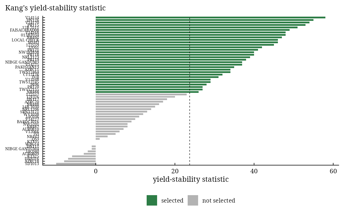
Kang's yield-stability statistic. Rank the means in ascending order (the highest mean gets rank $G$); with $LSD = t_{0.025, f_e}\sqrt{2s^2/(BE)}$ add +1, +2 or +3 when the mean exceeds the grand mean by less than one, at least one, or at least two LSD, and -1, -2 or -3 when it is below it by less than one, at least one, or at least two LSD; add the stability rating -8, -4 or -2 when $\sigma^2_i$ is significant at 0.01, 0.05 or alpha (0 otherwise). Genotypes with $YS_i$ above the mean of $YS$ are selected.

Changes from the earlier version. The stability parameters were divided by the number of replicates (the means, variances and coefficients of variation too); the pooled error had $(G - 1)^2E$ degrees of freedom; the stability rating for significance at alpha was +2 instead of -2; the LSD used a one-sided $t$; a covariate given in .envCov was used plot by plot instead of once per environment. All are corrected.

References

Shukla, G. K. (1972). Some statistical aspects of partitioning genotype-environmental components of variability. Heredity, 29(2), 237–245. doi:10.1038/hdy.1972.87

Kang, M. S. and Pham, H. N. (1991). Simultaneous selection for high yielding and stable crop genotypes. Agronomy Journal, 83(1), 161–165. doi:10.2134/agronj1991.00021962008300010037x

Kang, M. S. (1993). Simultaneous selection for yield and stability in crop performance trials: consequences for growers. Agronomy Journal, 85(3), 754–757.

Author

Muhammad Yaseen (myaseen208@gmail.com), Kent M. Eskridge (keskridge1@unl.edu)

Examples

data(ge_data)
fit <-
  stab_par(
      .data   = ge_data
    , .y      = Yield
    , .rep    = Rep
    , .gen    = Gen
    , .env    = Env
    , alpha   = 0.1
    , .envCov = NULL
    )
fit$ANOVA
#>                  Df    Sum Sq  Mean Sq  F value    Pr(>F)    
#> Total           659 536939402                                
#> Gen              59  71662431  1214617   3.7143 3.937e-16 ***
#> Env              10 263940496 26394050 266.1568 < 2.2e-16 ***
#> Gen x Env       590 201336476   341248   3.4411 < 2.2e-16 ***
#>   Heterogeneity  59  27695329   469412   1.4355   0.02256 *  
#>   Residual      531 173641147   327008   3.2975 < 2.2e-16 ***
#> Pooled error    649  64359568    99167                       
#> ---
#> Signif. codes:  0 ‘***’ 0.001 ‘**’ 0.01 ‘*’ 0.05 ‘.’ 0.1 ‘ ’ 1
head(fit$SimultSel)
#>             Gen     Mean  Rank Adjustment Adj.Rank     Sigma Stab.Rating   YSi
#>          <char>    <num> <int>      <int>    <int>     <num>       <int> <int>
#> 1:       V14154 4364.727    56          2       58  58121.11           0    58
#> 2:        DN126 4480.864    60          3       63 231116.61          -8    55
#> 3:       V14170 4463.818    59          3       62 199533.08          -8    54
#> 4:        PR115 4444.273    58          3       61 122904.01          -8    53
#> 5:     12B.2511 4414.409    57          2       59 255149.62          -8    51
#> 6: FAISALABAD08 4360.591    55          2       57 257374.96          -8    49
#>    Select
#>    <char>
#> 1:      +
#> 2:      +
#> 3:      +
#> 4:      +
#> 5:      +
#> 6:      +
plot(x = fit, which = c("ys", "sigma")[1])