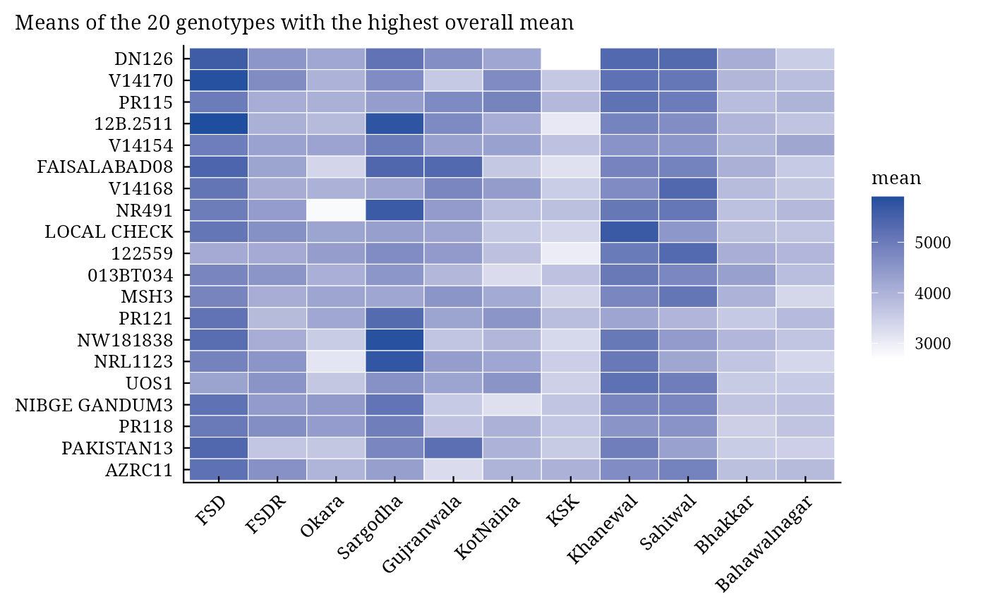
ge_means() tabulates the mean of every genotype in every environment, the genotype and environment means,
and the ranking of the genotypes within each environment, which shows at a glance whether the best genotypes
change from one environment to another (crossover interaction).
Value
An object of class c("stab_ge_means", "stab_result", "list") with the components of earlier
versions:
ge_meansdata.table, genotypes in rows and environments in columns.ge_means_matthe same as a matrix.
g_means,e_meansdata.tables of genotype and environment means.ge_rankscharacter matrix, environments in rows: the genotypes in decreasing order of mean.
and a new one:
rank_cormatrix of Spearman's rank correlations between environments.
Methods: print(), summary(), plot() (which = c("heatmap", "ranks")),
stab_interpret().
Details
\(\bar{y}_{ij}\) is the mean of genotype \(i\) in environment \(j\); \(\bar{y}_{i\cdot}\)
and \(\bar{y}_{\cdot j}\) are the means of the table's rows and columns (with missing plots, the means of
the cell means). Row \(j\) of ge_ranks lists the genotypes of environment \(j\) from the highest
mean down. The new component rank_cor holds Spearman's rank correlations of the genotype means between
pairs of environments; low or negative correlations indicate crossover interaction.
Change from the earlier version. g_means and e_means were in the order of the data; they
are now in the order of the levels (as the rows and columns of ge_means_mat).
See also
ge_effects, stab_fox, stab_interpret
Other stability analyses:
add_anova(),
ammi(),
ammi_biplot(),
er_anova(),
ge_effects(),
gge_biplot(),
indiv_anova(),
stab_asv(),
stab_dist(),
stab_eskridge(),
stab_fox(),
stab_huehn(),
stab_kang(),
stab_masv(),
stab_measures(),
stab_par(),
stab_reg(),
stab_reliability(),
stab_superiority()
Author
Muhammad Yaseen (myaseen208@gmail.com), Kent M. Eskridge (keskridge1@unl.edu)
Examples
data(ge_data)
fit <-
  ge_means(
      .data = ge_data
    , .y    = Yield
    , .gen  = Gen
    , .env  = Env
    )
fit$ge_ranks[, 1:5]
#>              1               2              3            4
#> FSD          "12B.2511"      "V14170"       "DN126"      "PR120"
#> FSDR         "V14170"        "PR119"        "PR118"      "QS3"
#> Okara        "NIBGE GANDUM3" "V13348"       "PR118"      "122559"
#> Sargodha     "NW181838"      "12B.2511"     "NRL1123"    "NR491"
#> Gujranwala   "IVII"          "FAISALABAD08" "PAKISTAN13" "V14168"
#> KotNaina     "PR115"         "V14170"       "WV1038"     "UOS1"
#> KSK          "NR448"         "12FJ26"       "AZRC11"     "BARDC1016"
#> Khanewal     "LOCAL CHECK"   "DN126"        "UOS1"       "V14170"
#> Sahiwal      "V14168"        "DN126"        "122559"     "MSH3"
#> Bhakkar      "V14225"        "013BT034"     "BARDC1016"  "14C036"
#> Bahawalnagar "V14154"        "KT335"        "V14225"     "PR115"
#>              5
#> FSD          "FAISALABAD08"
#> FSDR         "LOCAL CHECK"
#> Okara        "BARDC1016"
#> Sargodha     "AUR0810"
#> Gujranwala   "PR115"
#> KotNaina     "PR121"
#> KSK          "CT12176"
#> Khanewal     "PR115"
#> Sahiwal      "NR491"
#> Bhakkar      "DN126"
#> Bahawalnagar "TWS12464"
plot(x = fit, which = c("heatmap", "ranks")[1])