indiv_anova() analyses each environment of a multi-environment trial on its own, as a randomized complete
block experiment, and tests whether the error variances of the environments are homogeneous, which the pooled
error of the combined analysis (add_anova) assumes.
Usage
indiv_anova(.data, .y, .rep, .gen, .env)

# Default S3 method
indiv_anova(.data, .y, .rep, .gen, .env)
Arguments
- .data
a data frame (or
data.table) with one row per plot.- .y
response: a column of
.datagiven by name (.y = Yieldor.y = "Yield") or a numeric vector of lengthnrow(.data).- .rep
replicate (block within environment): a column of
.dataor a vector, as for.y.- .gen
genotype: a column of
.dataor a vector, as for.y.- .env
environment: a column of
.dataor a vector, as for.y.
Value
An object of class c("stab_indiv_anova", "stab_result", "list"): as in earlier versions, one
component per environment, named "ANOVA", a dash and the environment (see names(x)), with the summary.aov table of that
environment (lines Rep, Gen, Residuals); then two new components:
Summarydata frame, one row per environment:
Env,Mean,CV(percent),MSE,Df.error,F.Gen,p.Gen.Homogeneitydata frame: Bartlett's
Chisq,Df,p.value, andRatio(largest over smallest error mean square).
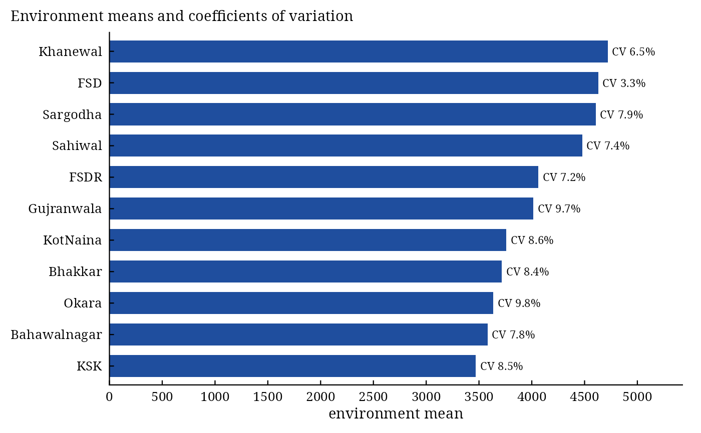
Methods: print(), summary(), plot() (environment means with their CV, which =
"means"; error mean squares, which = "error"), stab_interpret().
Details
In environment \(j\) the model is \(y_{ik} = \mu + b_k + g_i + \varepsilon_{ik}\), with \(B - 1\) degrees of freedom for replicates, \(G - 1\) for genotypes and \(f_j = (G - 1)(B - 1)\) for the error \(s^2_j\). The coefficient of variation is \(100\,s_j/\bar{y}_{\cdot j}\). Bartlett's test of equal error variances is $$\chi^2 = \frac{f\ln\bar{s}^2 - \sum_j f_j\ln s^2_j}{1 + \frac{1}{3(E - 1)}\left(\sum_j \frac{1}{f_j} - \frac{1}{f}\right)}, \qquad f = \sum_j f_j,\; \bar{s}^2 = \frac{\sum_j f_j s^2_j}{f},$$ on \(E - 1\) degrees of freedom; the ratio of the largest to the smallest error mean square is also given (a ratio below about 3 is commonly taken as acceptable for pooling).
Change from the earlier version. The analysis in each environment now includes the replicates (a randomized complete block analysis); the earlier version fitted genotypes only, so its error contained the replicate variation and its \(F\) tests were too small.
References
Bartlett, M. S. (1937). Properties of sufficiency and statistical tests. Proceedings of the Royal Society of London, Series A, 160(901), 268–282. doi:10.1098/rspa.1937.0109
Gomez, K. A. and Gomez, A. A. (1984). Statistical Procedures for Agricultural Research, 2nd edition. John Wiley and Sons, New York.
See also
Other stability analyses:
add_anova(),
ammi(),
ammi_biplot(),
er_anova(),
ge_effects(),
ge_means(),
gge_biplot(),
stab_asv(),
stab_dist(),
stab_eskridge(),
stab_fox(),
stab_huehn(),
stab_kang(),
stab_masv(),
stab_measures(),
stab_par(),
stab_reg(),
stab_reliability(),
stab_superiority()
Author
Muhammad Yaseen (myaseen208@gmail.com), Kent M. Eskridge (keskridge1@unl.edu)
Examples
data(ge_data)
fit <-
  indiv_anova(
      .data = ge_data
    , .y    = Yield
    , .rep  = Rep
    , .gen  = Gen
    , .env  = Env
    )
fit$Summary
#>             Env     Mean       CV       MSE Df.error     F.Gen        p.Gen
#> 1           FSD 4629.308 3.310148  23481.57       59 32.859696 9.777146e-30
#> 2          FSDR 4063.192 7.219829  86057.45       59  2.761218 7.071620e-05
#> 3         Okara 3634.433 9.816853 127296.96       59  3.568674 1.206599e-06
#> 4      Sargodha 4605.117 7.929968 133359.54       59  4.878042 3.670660e-09
#> 5    Gujranwala 4014.283 9.678154 150938.88       59  4.700962 7.608923e-09
#> 6      KotNaina 3759.633 8.606654 104703.14       59  4.320895 3.845328e-08
#> 7           KSK 3469.967 8.509432  87187.01       59  3.477938 1.870247e-06
#> 8      Khanewal 4718.567 6.465435  93071.27       59  2.754444 7.328681e-05
#> 9       Sahiwal 4477.833 7.381166 109241.03       59  4.051051 1.274773e-07
#> 10      Bhakkar 3714.667 8.415070  97713.64       59  1.885585 8.069768e-03
#> 11 Bahawalnagar 3581.325 7.787843  77789.65       59  2.117464 2.279749e-03
fit$Homogeneity
#>      Chisq Df     p.value    Ratio
#> 1 53.65762 10 5.61929e-08 6.427973
plot(x = fit, which = c("means", "error")[1])