1 Decision Making for Two Samples

TipMajor Themes of Chapter 5
  • Two-Sample Comparisons: Comparing parameters between two populations or treatments

  • Paired vs. Independent Samples: Understanding when to use different comparison methods

  • Variance Comparisons: Testing equality of variances using F-tests

  • Proportion Comparisons: Comparing success rates between two groups

  • Introduction to ANOVA: Extending two-sample methods to multiple samples

ImportantLearning Objectives

After careful study of this chapter, you should be able to do the following:

  1. Test hypotheses and construct confidence intervals for the difference between two means when variances are known and unknown.

  2. Understand and apply the pooled variance procedure for two-sample t-tests.

  3. Conduct and interpret paired t-tests for dependent samples.

  4. Test hypotheses and construct confidence intervals for the ratio of two variances using F-tests.

  5. Compare two population proportions using appropriate statistical methods.

  6. Calculate sample sizes and power for two-sample tests.

  7. Understand the basic concepts of Analysis of Variance (ANOVA).

  8. Distinguish between completely randomized and randomized complete block experimental designs.

1.1 Introduction

NoteTwo-Sample Problems

Many engineering problems involve comparing two populations, processes, or treatments. Common scenarios include:

  • Comparing the mean strength of materials from two suppliers

  • Testing whether a new manufacturing process reduces defect rates

  • Evaluating if a design modification improves performance

  • Comparing measurements before and after a process change

The choice of statistical method depends on:

  • Whether samples are independent or paired

  • Whether population variances are known or unknown

  • Whether variances can be assumed equal or unequal

1.2 Inference on the Means of Two Populations, Variances Known

1.2.1 Hypothesis Testing on the Difference in Means

NoteTwo-Sample Z-Test (σ₁, σ₂ known)

When both population variances are known, the test statistic for testing H₀: μ₁ = μ₂ is:

Z_0 = \frac{(\overline{X_1} - \overline{X_2}) - (\mu_1 - \mu_2)}{\sqrt{\frac{\sigma_1^2}{n_1} + \frac{\sigma_2^2}{n_2}}}

Under H₀: μ₁ - μ₂ = 0, Z₀ ~ N(0,1)

Common Hypothesis Tests:

  • Two-sided: H₀: μ₁ = μ₂ vs H₁: μ₁ ≠ μ₂

  • One-sided: H₀: μ₁ ≤ μ₂ vs H₁: μ₁ > μ₂

  • One-sided: H₀: μ₁ ≥ μ₂ vs H₁: μ₁ < μ₂

1.2.2 Example: Comparing Two Manufacturing Processes

NoteExample

A company wants to compare the tensile strength of cables produced by two different machines. Machine 1 produces cables with σ₁ = 12 psi, and Machine 2 with σ₂ = 10 psi. Random samples yield:

[1] "Cable Strength Data Summary by Machine:"
     machine     n      Min       Q1   Median     Mean       Q3      Max
      <char> <int>    <num>    <num>    <num>    <num>    <num>    <num>
1: Machine_1    20 221.4006 239.0774 246.4398 246.6995 251.5847 266.4430
2: Machine_2    25 221.1331 231.0529 235.9208 238.0735 246.2158 259.6896
          SD       Var
       <num>     <num>
1: 11.671984 136.23521
2:  9.449202  89.28741
library(collapse)
library(data.table)
library(ggplot2)
library(scales)
library(kableExtra)
library(gridExtra)
library(tidyr)

# Cable strength comparison (two-sample Z-test, sigma known)
set.seed(123)
cable_data <- data.table(
  machine = rep(c("Machine_1", "Machine_2"), c(20, 25)),
  strength = c(rnorm(20, mean = 245, sd = 12), rnorm(25, mean = 238, sd = 10))
)

# Summary statistics using collapse functions
cable_summary <- cable_data %>% 
  fgroup_by(machine) %>% 
  fsummarise(
    n = fnobs(strength),
    Min = fmin(strength),
    Q1 = fquantile(strength, 0.25),
    Median = fmedian(strength),
    Mean = fmean(strength),
    Q3 = fquantile(strength, 0.75),
    Max = fmax(strength),
    SD = fsd(strength),
    Var = fvar(strength)
  )

print("Cable Strength Data Summary by Machine:")
print(cable_summary)

# Write data to CSV for download
fwrite(cable_data, "data/cable_strength.csv")

Test H₀: μ₁ = μ₂ vs H₁: μ₁ ≠ μ₂ at α = 0.05.

Manual Calculation:

Given: n₁ = 20, x̄₁ = 245, σ₁ = 12, n₂ = 25, x̄₂ = 238, σ₂ = 10

  1. Test Statistic: Z_0 = \frac{(245 - 238) - 0}{\sqrt{\frac{12^2}{20} + \frac{10^2}{25}}} = \frac{7}{\sqrt{7.2 + 4}} = \frac{7}{3.35} = 2.09

  2. Critical Value: z₀.₀₂₅ = 1.96

  3. Decision: |Z₀| = 2.09 > 1.96, so reject H₀

[1] "Two-Sample Z-Test Results:"
                     Test_Type    n1    n2 xbar1  xbar2 sigma1 sigma2 Pooled_SE
                        <char> <int> <int> <num>  <num>  <num>  <num>     <num>
1: Two-sample Z-test (σ known)    20    25 246.7 238.07     12     10     3.347
   Z_Statistic P_Value Alpha Z_Critical  Decision
         <num>   <num> <num>      <num>    <char>
1:      2.5775    0.01  0.05       1.96 Reject H0
                          Conclusion
                              <char>
1: Means are significantly different
# Two-sample Z-test (manual and R calculations)
# Known population standard deviations
sigma1 <- 12
sigma2 <- 10
alpha <- 0.05

# Extract sample statistics
machine1_data <- cable_data[machine == "Machine_1"]
machine2_data <- cable_data[machine == "Machine_2"]

n1 <- fnobs(machine1_data$strength)
n2 <- fnobs(machine2_data$strength)
xbar1 <- fmean(machine1_data$strength)
xbar2 <- fmean(machine2_data$strength)

# Manual calculation
pooled_se <- sqrt((sigma1^2)/n1 + (sigma2^2)/n2)
z_stat <- (xbar1 - xbar2) / pooled_se
p_value_z <- 2 * (1 - pnorm(abs(z_stat)))  # Two-sided test
z_critical <- qnorm(1 - alpha/2)

# Test results
z_test_results <- data.table(
  Test_Type = "Two-sample Z-test (σ known)",
  n1 = n1,
  n2 = n2,
  xbar1 = round(xbar1, 2),
  xbar2 = round(xbar2, 2),
  sigma1 = sigma1,
  sigma2 = sigma2,
  Pooled_SE = round(pooled_se, 3),
  Z_Statistic = round(z_stat, 4),
  P_Value = round(p_value_z, 4),
  Alpha = alpha,
  Z_Critical = round(z_critical, 3),
  Decision = ifelse(abs(z_stat) > z_critical, "Reject H0", "Fail to reject H0"),
  Conclusion = ifelse(p_value_z < alpha, 
                     "Means are significantly different", 
                     "No significant difference in means")
)

print("Two-Sample Z-Test Results:")
print(z_test_results)

1.2.3 Type II Error and Choice of Sample Size

NotePower and Sample Size for Two-Sample Z-Test

Type II Error: For a specific difference δ = |μ₁ - μ₂|:

\beta = P\left(-z_{\alpha/2} - \frac{\delta}{\sqrt{\frac{\sigma_1^2}{n_1} + \frac{\sigma_2^2}{n_2}}} \leq Z \leq z_{\alpha/2} - \frac{\delta}{\sqrt{\frac{\sigma_1^2}{n_1} + \frac{\sigma_2^2}{n_2}}}\right)

Sample Size: For equal sample sizes (n₁ = n₂ = n):

n = \frac{(z_{\alpha/2} + z_\beta)^2(\sigma_1^2 + \sigma_2^2)}{\delta^2}

1.2.4 Example: Power Analysis

Figure 1: Power curves for two-sample Z-test
# Power curves for two-sample Z-test
delta_values <- seq(0, 15, by = 0.5)
sample_sizes <- c(10, 20, 30, 50)
alpha_power <- 0.05
sigma1_power <- 12
sigma2_power <- 10

# Function to calculate power for two-sample Z-test
calculate_power_two_sample <- function(delta, n1, n2, sigma1, sigma2, alpha) {
  se <- sqrt(sigma1^2/n1 + sigma2^2/n2)
  z_alpha2 <- qnorm(1 - alpha/2)
  
  # Power for two-sided test
  power <- 1 - pnorm(z_alpha2 - delta/se) + pnorm(-z_alpha2 - delta/se)
  return(power)
}

# Generate power curve data
power_curve_data <- data.table()
for(n_val in sample_sizes) {
  for(delta in delta_values) {
    power_val <- calculate_power_two_sample(delta, n_val, n_val, sigma1_power, sigma2_power, alpha_power)
    power_curve_data <- rbind(power_curve_data, 
                             data.table(delta = delta, n = factor(n_val), power = power_val))
  }
}

# Plot power curves
ggplot(data = power_curve_data, mapping = aes(x = delta, y = power, color = n)) +
  geom_line(linewidth = 1.2) +
  geom_hline(yintercept = 0.8, linetype = "dotted", alpha = 0.7) +
  annotate("text", x = 12, y = 0.82, label = "Power = 0.8", hjust = 0) +
  scale_x_continuous(breaks = pretty_breaks(n = 8)) +
  scale_y_continuous(breaks = pretty_breaks(n = 6), limits = c(0, 1)) +
  labs(
    x = "True Difference in Means (δ = |μ₁ - μ₂|)",
    y = "Power (1 - β)",
    color = "Sample Size\n(each group)",
    title = "Power Curves for Two-Sample Z-Test",
    subtitle = "H₀: μ₁ = μ₂ vs H₁: μ₁ ≠ μ₂, α = 0.05, σ₁ = 12, σ₂ = 10"
  ) +
  theme_classic() +
  theme(
    plot.title = element_text(hjust = 0.5),
    plot.subtitle = element_text(hjust = 0.5),
    legend.position = "right"
  )

1.2.5 Confidence Interval on the Difference in Means

NoteConfidence Interval for μ₁ - μ₂ (σ₁, σ₂ known)

A 100(1-α)% confidence interval for μ₁ - μ₂:

(\overline{x_1} - \overline{x_2}) \pm z_{\alpha/2}\sqrt{\frac{\sigma_1^2}{n_1} + \frac{\sigma_2^2}{n_2}}

[1] "95% Confidence Interval for Difference in Means (σ known):"
   Parameter Confidence_Level Difference Standard_Error Z_Critical Margin_Error
      <char>           <char>      <num>          <num>      <num>        <num>
1:   μ₁ - μ₂              95%       8.63          3.347       1.96        6.559
   Lower_Bound Upper_Bound Width
         <num>       <num> <num>
1:        2.07       15.19 13.12
                                         Interpretation
                                                 <char>
1: 95% confident that μ₁ - μ₂ is between 2.07 and 15.19
# Confidence interval for difference in means (sigma known)
margin_error_z <- z_critical * pooled_se
ci_lower_z <- (xbar1 - xbar2) - margin_error_z
ci_upper_z <- (xbar1 - xbar2) + margin_error_z

z_ci_results <- data.table(
  Parameter = "μ₁ - μ₂",
  Confidence_Level = "95%",
  Difference = round(xbar1 - xbar2, 2),
  Standard_Error = round(pooled_se, 3),
  Z_Critical = round(z_critical, 3),
  Margin_Error = round(margin_error_z, 3),
  Lower_Bound = round(ci_lower_z, 2),
  Upper_Bound = round(ci_upper_z, 2),
  Width = round(ci_upper_z - ci_lower_z, 2),
  Interpretation = paste("95% confident that μ₁ - μ₂ is between", 
                        round(ci_lower_z, 2), "and", round(ci_upper_z, 2))
)

print("95% Confidence Interval for Difference in Means (σ known):")
print(z_ci_results)

1.3 Inference on the Means of Two Populations, Variances Unknown

1.3.1 Hypothesis Testing on the Difference in Means

NoteTwo-Sample t-Test (σ₁, σ₂ unknown)

When population variances are unknown, we must consider two cases:

Case 1: Equal Variances (σ₁² = σ₂²)

  • Use pooled variance:

S_p^2 = \frac{(n_1-1)S_1^2 + (n_2-1)S_2^2}{n_1 + n_2 - 2}

  • Test statistic:

T_0 = \frac{\overline{X_1} - \overline{X_2}}{S_p\sqrt{\frac{1}{n_1} + \frac{1}{n_2}}}

  • Degrees of freedom: ν = n₁ + n₂ - 2

Case 2: Unequal Variances (σ₁² ≠ σ₂²)

  • Welch’s t-test

  • Test statistic:

T_0 = \frac{\overline{X_1} - \overline{X_2}}{\sqrt{\frac{S_1^2}{n_1} + \frac{S_2^2}{n_2}}}

  • Degrees of freedom:

\nu = \frac{(\frac{S_1^2}{n_1} + \frac{S_2^2}{n_2})^2}{\frac{S_1^4}{n_1^2(n_1-1)} + \frac{S_2^4}{n_2^2(n_2-1)}}

1.3.2 Example: Comparing Material Strength

NoteExample

Compare the breaking strength of two types of plastic. Random samples give:

[1] "Plastic Strength Data Summary by Type:"
     type     n      Min       Q1   Median     Mean       Q3      Max        SD
   <char> <int>    <num>    <num>    <num>    <num>    <num>    <num>     <num>
1: Type_A    15 150.6854 155.8163 167.2005 163.4680 169.8374 176.0622  8.599716
2: Type_B    18 139.6099 152.5444 156.1428 158.8415 170.5125 178.5483 11.920081
         Var  SE_Mean
       <num>    <num>
1:  73.95511 2.220437
2: 142.08832 2.809590
# Plastic strength comparison (two-sample t-test, sigma unknown)
set.seed(456)
plastic_data <- data.table(
  type = rep(c("Type_A", "Type_B"), c(15, 18)),
  strength = c(rnorm(15, mean = 162.5, sd = 8.2), rnorm(18, mean = 157.8, sd = 9.1))
)

# Summary statistics
plastic_summary <- plastic_data %>% 
  fgroup_by(type) %>% 
  fsummarise(
    n = fnobs(strength),
    Min = fmin(strength),
    Q1 = fquantile(strength, 0.25),
    Median = fmedian(strength),
    Mean = fmean(strength),
    Q3 = fquantile(strength, 0.75),
    Max = fmax(strength),
    SD = fsd(strength),
    Var = fvar(strength),
    SE_Mean = fsd(strength) / sqrt(fnobs(strength))
  )

print("Plastic Strength Data Summary by Type:")
print(plastic_summary)

# Write data to CSV for download
fwrite(plastic_data, "data/plastic_strength.csv")

First, test for equal variances, then perform appropriate t-test.

Manual Calculation (assuming equal variances):

Given: n₁ = 15, x̄₁ = 162.5, s₁ = 8.2, n₂ = 18, x̄₂ = 157.8, s₂ = 9.1

  1. Pooled Variance: S_p^2 = \frac{(15-1)(8.2)^2 + (18-1)(9.1)^2}{15 + 18 - 2} = \frac{940.36 + 1408.57}{31} = 75.77

  2. Test Statistic: T_0 = \frac{162.5 - 157.8}{8.71\sqrt{\frac{1}{15} + \frac{1}{18}}} = \frac{4.7}{3.01} = 1.56

  3. Critical Value: t₀.₀₂₅,₃₁ = 2.040

  4. Decision: |T₀| = 1.56 < 2.040, so fail to reject H₀

[1] "F-test for equal variances: F = 0.52 , p-value = 0.2229"
[1] "Two-Sample t-Test Results (Equal Variances):"
                             Test_Type    n1    n2  xbar1  xbar2    s1    s2
                                <char> <int> <int>  <num>  <num> <num> <num>
1: Two-sample t-test (equal variances)    15    18 163.47 158.84   8.6 11.92
   Pooled_SD SE_Difference t_Statistic    df P_Value Alpha t_Critical
       <num>         <num>       <num> <num>   <num> <num>      <num>
1:     10.55         3.689      1.2543    31  0.2191  0.05       2.04
            Decision                         Conclusion
              <char>                             <char>
1: Fail to reject H0 No significant difference in means
[1] "R's t.test verification:"

    Two Sample t-test

data:  typeA_data$strength and typeB_data$strength
t = 1.2543, df = 31, p-value = 0.2191
alternative hypothesis: true difference in means is not equal to 0
95 percent confidence interval:
 -2.896371 12.149429
sample estimates:
mean of x mean of y 
 163.4680  158.8415 
# Two-sample t-test with equal variances (manual and R calculations)
typeA_data <- plastic_data[type == "Type_A"]
typeB_data <- plastic_data[type == "Type_B"]

n1_t <- fnobs(typeA_data$strength)
n2_t <- fnobs(typeB_data$strength)
xbar1_t <- fmean(typeA_data$strength)
xbar2_t <- fmean(typeB_data$strength)
s1_t <- fsd(typeA_data$strength)
s2_t <- fsd(typeB_data$strength)

# Test for equal variances first (F-test)
f_stat_equal <- s1_t^2 / s2_t^2
df1_f <- n1_t - 1
df2_f <- n2_t - 1
p_value_f <- 2 * min(pf(f_stat_equal, df1_f, df2_f), 1 - pf(f_stat_equal, df1_f, df2_f))

print(paste("F-test for equal variances: F =", round(f_stat_equal, 3), ", p-value =", round(p_value_f, 4)))

# Assuming equal variances (pooled variance)
sp_squared <- ((n1_t - 1) * s1_t^2 + (n2_t - 1) * s2_t^2) / (n1_t + n2_t - 2)
sp <- sqrt(sp_squared)
se_pooled <- sp * sqrt(1/n1_t + 1/n2_t)

# Manual t-test calculation
t_stat <- (xbar1_t - xbar2_t) / se_pooled
df_t <- n1_t + n2_t - 2
p_value_t <- 2 * (1 - pt(abs(t_stat), df = df_t))
t_critical <- qt(1 - alpha/2, df = df_t)

# Test results
t_test_results <- data.table(
  Test_Type = "Two-sample t-test (equal variances)",
  n1 = n1_t,
  n2 = n2_t,
  xbar1 = round(xbar1_t, 2),
  xbar2 = round(xbar2_t, 2),
  s1 = round(s1_t, 2),
  s2 = round(s2_t, 2),
  Pooled_SD = round(sp, 2),
  SE_Difference = round(se_pooled, 3),
  t_Statistic = round(t_stat, 4),
  df = df_t,
  P_Value = round(p_value_t, 4),
  Alpha = alpha,
  t_Critical = round(t_critical, 3),
  Decision = ifelse(abs(t_stat) > t_critical, "Reject H0", "Fail to reject H0"),
  Conclusion = ifelse(p_value_t < alpha, 
                     "Means are significantly different", 
                     "No significant difference in means")
)

print("Two-Sample t-Test Results (Equal Variances):")
print(t_test_results)

# Using R's built-in t.test for verification
t_test_r <- t.test(typeA_data$strength, typeB_data$strength, var.equal = TRUE)
print("R's t.test verification:")
print(t_test_r)

1.3.3 Type II Error and Choice of Sample Size

NoteSample Size for Two-Sample t-Test

For equal sample sizes and equal variances:

n \approx \frac{2(t_{\alpha/2,\nu} + t_{\beta,\nu})^2 s_p^2}{\delta^2}

where ν = 2n - 2 and s_p² is estimated from pilot data.

1.3.4 Confidence Interval on the Difference in Means

NoteConfidence Interval for μ₁ - μ₂ (σ₁, σ₂ unknown)

Equal Variances:

(\overline{x_1} - \overline{x_2}) \pm t_{\alpha/2,n_1+n_2-2} \cdot S_p\sqrt{\frac{1}{n_1} + \frac{1}{n_2}}

Unequal Variances:

(\overline{x_1} - \overline{x_2}) \pm t_{\alpha/2,\nu} \sqrt{\frac{s_1^2}{n_1} + \frac{s_2^2}{n_2}}

[1] "95% Confidence Interval for Difference in Means (σ unknown):"
   Parameter Confidence_Level Difference Pooled_SD Standard_Error t_Critical
      <char>           <char>      <num>     <num>          <num>      <num>
1:   μ₁ - μ₂              95%       4.63     10.55          3.689       2.04
   Margin_Error Lower_Bound Upper_Bound Width
          <num>       <num>       <num> <num>
1:        7.523        -2.9       12.15 15.05
                                         Interpretation
                                                 <char>
1: 95% confident that μ₁ - μ₂ is between -2.9 and 12.15
[1] "Welch's t-test (unequal variances):"

    Welch Two Sample t-test

data:  typeA_data$strength and typeB_data$strength
t = 1.2919, df = 30.446, p-value = 0.2061
alternative hypothesis: true difference in means is not equal to 0
95 percent confidence interval:
 -2.682527 11.935585
sample estimates:
mean of x mean of y 
 163.4680  158.8415 
# Confidence interval for difference in means (sigma unknown)
margin_error_t <- t_critical * se_pooled
ci_lower_t <- (xbar1_t - xbar2_t) - margin_error_t
ci_upper_t <- (xbar1_t - xbar2_t) + margin_error_t

t_ci_results <- data.table(
  Parameter = "μ₁ - μ₂",
  Confidence_Level = "95%",
  Difference = round(xbar1_t - xbar2_t, 2),
  Pooled_SD = round(sp, 2),
  Standard_Error = round(se_pooled, 3),
  t_Critical = round(t_critical, 3),
  Margin_Error = round(margin_error_t, 3),
  Lower_Bound = round(ci_lower_t, 2),
  Upper_Bound = round(ci_upper_t, 2),
  Width = round(ci_upper_t - ci_lower_t, 2),
  Interpretation = paste("95% confident that μ₁ - μ₂ is between", 
                        round(ci_lower_t, 2), "and", round(ci_upper_t, 2))
)

print("95% Confidence Interval for Difference in Means (σ unknown):")
print(t_ci_results)

# Welch's t-test (unequal variances) for comparison
welch_test <- t.test(typeA_data$strength, typeB_data$strength, var.equal = FALSE)
print("Welch's t-test (unequal variances):")
print(welch_test)

1.4 The Paired t-Test

NotePaired t-Test

When observations come in natural pairs (before/after, matched subjects, etc.), use the paired t-test:

  1. Calculate differences: d_i = x₁ᵢ - x₂ᵢ

  2. Test statistic:

T_0 = \frac{\overline{d} - \mu_d}{S_d/\sqrt{n}}

  1. Degrees of freedom: ν = n - 1

Where:

  • \overline{d} = \frac{1}{n}\sum_{i=1}^n d_i

  • S_d^2 = \frac{1}{n-1}\sum_{i=1}^n (d_i - \overline{d})^2

Assumptions:

  • Differences are normally distributed

  • Pairs are independent

1.4.1 Example: Before/After Comparison

NoteExample

A manufacturing process improvement is tested on 12 production lines. Measure output before and after the improvement:

[1] "Process Improvement Paired Data Summary:"
       n Mean_Before Mean_After Mean_Difference SD_Before SD_After
   <int>       <num>      <num>           <num>     <num>    <num>
1:    12    81.70922   89.14206        7.432843   6.36605 4.794191
   SD_Difference SE_Difference Min_Difference Max_Difference
           <num>         <num>          <num>          <num>
1:      6.906354      1.993693      -2.023308        19.6769
[1] "Individual Differences:"
    line_id   before    after difference
      <int>    <num>    <num>      <num>
 1:       1 89.19277 88.91711 -0.2756677
 2:       2 66.91386 86.59075 19.6768963
 3:       3 84.84256 97.20931 12.3667432
 4:       4 86.46512 84.44181 -2.0233083
 5:       5 82.10919 93.42153 11.3123453
 6:       6 81.12413 85.69777  4.5736465
 7:       7 79.66950 91.82031 12.1508159
 8:       8 83.60425 84.41997  0.8157253
 9:       9 76.91232 84.98462  8.0723014
10:      10 90.91757 95.37602  4.4584503
11:      11 81.78163 83.81734  2.0357137
12:      12 76.97776 93.00821 16.0304489
# Process improvement paired t-test example
set.seed(789)
process_data <- data.table(
  line_id = 1:12,
  before = rnorm(12, mean = 85, sd = 8),
  after = rnorm(12, mean = 90.25, sd = 7.5)
)

# Calculate differences
process_data[, difference := after - before]

# Summary statistics for paired data
paired_summary <- process_data %>% 
  fsummarise(
    n = fnobs(difference),
    Mean_Before = fmean(before),
    Mean_After = fmean(after),
    Mean_Difference = fmean(difference),
    SD_Before = fsd(before),
    SD_After = fsd(after),
    SD_Difference = fsd(difference),
    SE_Difference = fsd(difference) / sqrt(fnobs(difference)),
    Min_Difference = fmin(difference),
    Max_Difference = fmax(difference)
  )

print("Process Improvement Paired Data Summary:")
print(paired_summary)

# Individual differences
differences_table <- process_data[, .(line_id, before, after, difference)]
print("Individual Differences:")
print(differences_table)

# Write data to CSV for download
fwrite(process_data, "data/process_improvement.csv")

Test H₀: μ_d = 0 vs H₁: μ_d > 0 at α = 0.05.

Manual Calculation:

Calculate differences: d_i = After_i - Before_i

If d̄ = 5.25 and s_d = 3.2:

  1. Test Statistic: T_0 = \frac{5.25 - 0}{3.2/\sqrt{12}} = \frac{5.25}{0.924} = 5.68

  2. Critical Value: t₀.₀₅,₁₁ = 1.796

  3. Decision: T₀ = 5.68 > 1.796, so reject H₀

[1] "Paired t-Test Results:"
       Test_Type n_pairs Mean_Difference SD_Difference SE_Difference
          <char>   <int>           <num>         <num>         <num>
1: Paired t-test      12           7.433         6.906         1.994
   Null_Difference t_Statistic    df P_Value Alpha t_Critical  Decision
             <num>       <num> <num>   <num> <num>      <num>    <char>
1:               0      3.7282    11  0.0017  0.05      1.796 Reject H0
                         Conclusion
                             <char>
1: Significant improvement detected
[1] "R's paired t.test verification:"

    Paired t-test

data:  process_data$after and process_data$before
t = 3.7282, df = 11, p-value = 0.001667
alternative hypothesis: true mean difference is greater than 0
95 percent confidence interval:
 3.8524    Inf
sample estimates:
mean difference 
       7.432843 
[1] "95% CI for mean difference: [ 3.045 ,  11.821 ]"
# Paired t-test (manual and R calculations)
n_paired <- fnobs(process_data$difference)
d_bar <- fmean(process_data$difference)
s_d <- fsd(process_data$difference)
mu_d0 <- 0  # Null hypothesis: no difference

# Manual calculation
t_stat_paired <- (d_bar - mu_d0) / (s_d / sqrt(n_paired))
df_paired <- n_paired - 1
p_value_paired <- 1 - pt(t_stat_paired, df = df_paired)  # One-sided upper test
t_critical_paired <- qt(1 - alpha, df = df_paired)

# Test results
paired_test_results <- data.table(
  Test_Type = "Paired t-test",
  n_pairs = n_paired,
  Mean_Difference = round(d_bar, 3),
  SD_Difference = round(s_d, 3),
  SE_Difference = round(s_d / sqrt(n_paired), 3),
  Null_Difference = mu_d0,
  t_Statistic = round(t_stat_paired, 4),
  df = df_paired,
  P_Value = round(p_value_paired, 4),
  Alpha = alpha,
  t_Critical = round(t_critical_paired, 3),
  Decision = ifelse(t_stat_paired > t_critical_paired, "Reject H0", "Fail to reject H0"),
  Conclusion = ifelse(p_value_paired < alpha, 
                     "Significant improvement detected", 
                     "No significant improvement")
)

print("Paired t-Test Results:")
print(paired_test_results)

# Using R's paired t.test for verification
paired_test_r <- t.test(process_data$after, process_data$before, paired = TRUE, alternative = "greater")
print("R's paired t.test verification:")
print(paired_test_r)

# Confidence interval for mean difference
t_critical_ci_paired <- qt(1 - alpha/2, df = df_paired)
margin_error_paired <- t_critical_ci_paired * (s_d / sqrt(n_paired))
ci_lower_paired <- d_bar - margin_error_paired
ci_upper_paired <- d_bar + margin_error_paired

print(paste("95% CI for mean difference: [", round(ci_lower_paired, 3), ", ", round(ci_upper_paired, 3), "]"))
Figure 2: Paired t-test visualization
# Paired t-test visualization

# Create long format for plotting
process_long <- process_data %>%
  pivot_longer(cols = c(before, after), names_to = "time", values_to = "output") %>%
  data.table()

# Before/After comparison plot
p1 <- ggplot(data = process_long, mapping = aes(x = time, y = output, group = line_id)) +
  geom_line(color = "gray", alpha = 0.7) +
  geom_point(mapping = aes(color = time), size = 3) +
  scale_color_manual(values = c("before" = "red", "after" = "blue")) +
  labs(
    x = "Time Period",
    y = "Output",
    title = "Before/After Process Improvement",
    color = "Period"
  ) +
  theme_classic() +
  theme(plot.title = element_text(hjust = 0.5))

# Differences histogram
p2 <- ggplot(data = process_data, mapping = aes(x = difference)) +
  geom_histogram(bins = 8, fill = "lightblue", color = "black", alpha = 0.7) +
  geom_vline(xintercept = d_bar, color = "red", linetype = "dashed", linewidth = 1) +
  geom_vline(xintercept = 0, color = "black", linetype = "solid", linewidth = 1) +
  labs(
    x = "Difference (After - Before)",
    y = "Frequency",
    title = "Distribution of Differences"
  ) +
  theme_classic() +
  theme(plot.title = element_text(hjust = 0.5))

# Combine plots
grid.arrange(p1, p2, nrow = 1, ncol = 2)

1.5 Inference on the Ratio of Variances of Two Normal Populations

1.5.1 Hypothesis Testing on the Ratio of Two Variances

NoteF-Test for Equality of Variances

To test H₀: σ₁² = σ₂² vs H₁: σ₁² ≠ σ₂², use:

F_0 = \frac{S_1^2}{S_2^2}

Under H₀, F₀ ~ F_{n₁-1, n₂-1}

Convention: Put the larger sample variance in the numerator so F₀ ≥ 1.

Properties of F-distribution:

  • Always positive

  • Right-skewed

  • Approaches 1 as both df → ∞

  • F₁₋α,ν₁,ν₂ = 1/F_α,ν₂,ν₁

1.5.2 Example: Variance Comparison

NoteExample

Compare the variability in measurements from two instruments:

[1] "Instrument Comparison Data Summary:"
     instrument     n      Min       Q1   Median     Mean       Q3      Max
         <char> <int>    <num>    <num>    <num>    <num>    <num>    <num>
1: Instrument_1    16 23.17625 24.45219 25.33319 25.39453 25.69963 28.86313
2: Instrument_2    21 22.07273 24.18302 25.35367 25.00446 25.81188 26.85136
         SD      Var
      <num>    <num>
1: 1.522413 2.317741
2: 1.359890 1.849302
# Instrument comparison for F-test (variance comparison)
set.seed(321)
instrument_data <- data.table(
  instrument = rep(c("Instrument_1", "Instrument_2"), c(16, 21)),
  measurement = c(rnorm(16, mean = 25, sd = sqrt(2.5)), rnorm(21, mean = 25.2, sd = sqrt(1.8)))
)

# Summary statistics
instrument_summary <- instrument_data %>% 
  fgroup_by(instrument) %>% 
  fsummarise(
    n = fnobs(measurement),
    Min = fmin(measurement),
    Q1 = fquantile(measurement, 0.25),
    Median = fmedian(measurement),
    Mean = fmean(measurement),
    Q3 = fquantile(measurement, 0.75),
    Max = fmax(measurement),
    SD = fsd(measurement),
    Var = fvar(measurement)
  )

print("Instrument Comparison Data Summary:")
print(instrument_summary)

# Write data to CSV for download
fwrite(instrument_data, "data/instrument_comparison.csv")

Test H₀: σ₁² = σ₂² vs H₁: σ₁² ≠ σ₂² at α = 0.05.

Manual Calculation:

Given: n₁ = 16, s₁² = 2.5, n₂ = 21, s₂² = 1.8

  1. Test Statistic: F_0 = \frac{2.5}{1.8} = 1.39

  2. Critical Value: F₀.₀₂₅,₁₅,₂₀ = 2.57

  3. Decision: F₀ = 1.39 < 2.57, so fail to reject H₀

[1] "F-Test Results for Equality of Variances:"
                          Test_Type    n1    n2 s1_squared s2_squared
                             <char> <int> <int>      <num>      <num>
1: F-test for equality of variances    16    21     2.3177     1.8493
   Larger_Variance F_Statistic   df1   df2 P_Value Alpha F_Critical
            <char>       <num> <num> <num>   <num> <num>      <num>
1:    Instrument_1      1.2533    15    20   0.627  0.05      2.573
            Decision                             Conclusion
              <char>                                 <char>
1: Fail to reject H0 No significant difference in variances
[1] "R's var.test verification:"

    F test to compare two variances

data:  inst1_data$measurement and inst2_data$measurement
F = 1.2533, num df = 15, denom df = 20, p-value = 0.627
alternative hypothesis: true ratio of variances is not equal to 1
95 percent confidence interval:
 0.4870809 3.4539881
sample estimates:
ratio of variances 
          1.253306 
# F-test for equality of variances
inst1_data <- instrument_data[instrument == "Instrument_1"]
inst2_data <- instrument_data[instrument == "Instrument_2"]

n1_f <- fnobs(inst1_data$measurement)
n2_f <- fnobs(inst2_data$measurement)
s1_f_squared <- fvar(inst1_data$measurement)
s2_f_squared <- fvar(inst2_data$measurement)

# F-test (put larger variance in numerator)
if(s1_f_squared >= s2_f_squared) {
  f_stat <- s1_f_squared / s2_f_squared
  df1_f_test <- n1_f - 1
  df2_f_test <- n2_f - 1
  larger_var <- "Instrument_1"
} else {
  f_stat <- s2_f_squared / s1_f_squared
  df1_f_test <- n2_f - 1
  df2_f_test <- n1_f - 1
  larger_var <- "Instrument_2"
}

# Calculate p-value for two-sided test
p_value_f_test <- 2 * (1 - pf(f_stat, df1_f_test, df2_f_test))
f_critical <- qf(1 - alpha/2, df1_f_test, df2_f_test)

# Test results
f_test_results <- data.table(
  Test_Type = "F-test for equality of variances",
  n1 = n1_f,
  n2 = n2_f,
  s1_squared = round(s1_f_squared, 4),
  s2_squared = round(s2_f_squared, 4),
  Larger_Variance = larger_var,
  F_Statistic = round(f_stat, 4),
  df1 = df1_f_test,
  df2 = df2_f_test,
  P_Value = round(p_value_f_test, 4),
  Alpha = alpha,
  F_Critical = round(f_critical, 3),
  Decision = ifelse(f_stat > f_critical, "Reject H0", "Fail to reject H0"),
  Conclusion = ifelse(p_value_f_test < alpha, 
                     "Variances are significantly different", 
                     "No significant difference in variances")
)

print("F-Test Results for Equality of Variances:")
print(f_test_results)

# Using R's var.test for verification
var_test_r <- var.test(inst1_data$measurement, inst2_data$measurement)
print("R's var.test verification:")
print(var_test_r)

1.5.3 Confidence Interval on the Ratio of Two Variances

NoteConfidence Interval for σ₁²/σ₂²

A 100(1-α)% confidence interval for σ₁²/σ₂²:

\frac{s_1^2/s_2^2}{F_{\alpha/2,n_1-1,n_2-1}} \leq \frac{\sigma_1^2}{\sigma_2^2} \leq \frac{s_1^2/s_2^2}{F_{1-\alpha/2,n_1-1,n_2-1}}

Note: F₁₋α/₂,ν₁,ν₂ = 1/F_α/₂,ν₂,ν₁

[1] "95% Confidence Interval for Ratio of Variances:"
   Parameter Confidence_Level Sample_Ratio Lower_Bound Upper_Bound  Width
      <char>           <char>        <num>       <num>       <num>  <num>
1:   σ₁²/σ₂²              95%       1.2533      0.4871       3.454 2.9669
                                           Interpretation
                                                   <char>
1: 95% confident that σ₁²/σ₂² is between 0.4871 and 3.454
# Confidence interval for ratio of variances
f_alpha2_lower <- qf(alpha/2, df1_f_test, df2_f_test)
f_alpha2_upper <- qf(1 - alpha/2, df1_f_test, df2_f_test)

# Note: For CI, use original ratio without putting larger in numerator
ratio_original <- s1_f_squared / s2_f_squared
ci_lower_f <- ratio_original / f_alpha2_upper
ci_upper_f <- ratio_original / f_alpha2_lower

variance_ratio_ci <- data.table(
  Parameter = "σ₁²/σ₂²",
  Confidence_Level = "95%",
  Sample_Ratio = round(ratio_original, 4),
  Lower_Bound = round(ci_lower_f, 4),
  Upper_Bound = round(ci_upper_f, 4),
  Width = round(ci_upper_f - ci_lower_f, 4),
  Interpretation = paste("95% confident that σ₁²/σ₂² is between", 
                        round(ci_lower_f, 4), "and", round(ci_upper_f, 4))
)

print("95% Confidence Interval for Ratio of Variances:")
print(variance_ratio_ci)

1.6 Inference on Two Population Proportions

1.6.1 Hypothesis Testing on the Equality of Two Proportions

NoteTwo-Sample Z-Test for Proportions

To test H₀: p₁ = p₂, use the pooled estimate:

\hat{p} = \frac{x_1 + x_2}{n_1 + n_2}

Test Statistic:

Z_0 = \frac{\hat{p_1} - \hat{p_2}}{\sqrt{\hat{p}(1-\hat{p})(\frac{1}{n_1} + \frac{1}{n_2})}}

Conditions: n₁p̂ ≥ 5, n₁(1-p̂) ≥ 5, n₂p̂ ≥ 5, n₂(1-p̂) ≥ 5

1.6.2 Example: Comparing Defect Rates

NoteExample

Compare defect rates between two production lines:

[1] "Defect Rate Comparison Summary:"
     line sample_size defects  prop
   <char>       <num>   <num> <num>
1: Line_1         200      16 0.080
2: Line_2         250      14 0.056
[1] "Overall Summary:"
   Total_Items Total_Defects Line1_Rate Line2_Rate Overall_Rate
         <num>         <num>      <num>      <num>        <num>
1:         450            30       0.08      0.056   0.06666667
# Defect rate comparison (two-sample proportion test)
defect_comparison_data <- data.table(
  line = c("Line_1", "Line_2"),
  sample_size = c(200, 250),
  defects = c(16, 14),
  prop = c(16/200, 14/250)
)

# Summary
defect_summary <- defect_comparison_data %>% 
  fsummarise(
    Total_Items = fsum(sample_size),
    Total_Defects = fsum(defects),
    Line1_Rate = defects[1] / sample_size[1],
    Line2_Rate = defects[2] / sample_size[2],
    Overall_Rate = fsum(defects) / fsum(sample_size)
  )

print("Defect Rate Comparison Summary:")
print(defect_comparison_data)
print("Overall Summary:")
print(defect_summary)

# Write data to CSV for download
fwrite(defect_comparison_data, "data/defect_comparison.csv")

Test H₀: p₁ = p₂ vs H₁: p₁ ≠ p₂ at α = 0.05.

Manual Calculation:

Given: n₁ = 200, x₁ = 16, n₂ = 250, x₂ = 14

  1. Sample Proportions:

    • p̂₁ = 16/200 = 0.08

    • p̂₂ = 14/250 = 0.056

  2. Pooled Proportion: \hat{p} = \frac{16 + 14}{200 + 250} = \frac{30}{450} = 0.067

  3. Test Statistic: Z_0 = \frac{0.08 - 0.056}{\sqrt{0.067(0.933)(\frac{1}{200} + \frac{1}{250})}} = \frac{0.024}{0.024} = 1.00

  4. Decision: |Z₀| = 1.00 < 1.96, so fail to reject H₀

[1] "Large Sample Conditions:"
     Condition     Value    Met
        <char>     <num> <lgcl>
1:     n₁p̂ ≥ 5  13.33333   TRUE
2: n₁(1-p̂) ≥ 5 186.66667   TRUE
3:     n₂p̂ ≥ 5  16.66667   TRUE
4: n₂(1-p̂) ≥ 5 233.33333   TRUE
[1] "Two-Sample Proportion Test Results:"
                    Test_Type    n1    n2    x1    x2 p1_hat p2_hat p_pooled
                       <char> <num> <num> <num> <num>  <num>  <num>    <num>
1: Two-sample proportion test   200   250    16    14   0.08  0.056   0.0667
   SE_Difference Z_Statistic P_Value Alpha Z_Critical          Decision
           <num>       <num>   <num> <num>      <num>            <char>
1:        0.0237      1.0142  0.3105  0.05       1.96 Fail to reject H0
                                 Conclusion
                                     <char>
1: No significant difference in proportions
[1] "R's prop.test verification:"

    2-sample test for equality of proportions with continuity correction

data:  c(x1_prop, x2_prop) out of c(n1_prop, n2_prop)
X-squared = 0.67902, df = 1, p-value = 0.4099
alternative hypothesis: two.sided
95 percent confidence interval:
 -0.02768004  0.07568004
sample estimates:
prop 1 prop 2 
 0.080  0.056 
# Two-sample proportion test
n1_prop <- defect_comparison_data[line == "Line_1", sample_size]
n2_prop <- defect_comparison_data[line == "Line_2", sample_size]
x1_prop <- defect_comparison_data[line == "Line_1", defects]
x2_prop <- defect_comparison_data[line == "Line_2", defects]
p1_hat <- x1_prop / n1_prop
p2_hat <- x2_prop / n2_prop

# Pooled proportion
p_pooled <- (x1_prop + x2_prop) / (n1_prop + n2_prop)

# Check conditions
conditions <- data.table(
  Condition = c("n₁p̂ ≥ 5", "n₁(1-p̂) ≥ 5", "n₂p̂ ≥ 5", "n₂(1-p̂) ≥ 5"),
  Value = c(n1_prop * p_pooled, n1_prop * (1 - p_pooled), 
           n2_prop * p_pooled, n2_prop * (1 - p_pooled)),
  Met = c(n1_prop * p_pooled >= 5, n1_prop * (1 - p_pooled) >= 5,
         n2_prop * p_pooled >= 5, n2_prop * (1 - p_pooled) >= 5)
)

print("Large Sample Conditions:")
print(conditions)

# Manual calculation
se_prop <- sqrt(p_pooled * (1 - p_pooled) * (1/n1_prop + 1/n2_prop))
z_stat_prop <- (p1_hat - p2_hat) / se_prop
p_value_prop <- 2 * (1 - pnorm(abs(z_stat_prop)))  # Two-sided test
z_critical_prop <- qnorm(1 - alpha/2)

# Test results
prop_test_results <- data.table(
  Test_Type = "Two-sample proportion test",
  n1 = n1_prop,
  n2 = n2_prop,
  x1 = x1_prop,
  x2 = x2_prop,
  p1_hat = round(p1_hat, 4),
  p2_hat = round(p2_hat, 4),
  p_pooled = round(p_pooled, 4),
  SE_Difference = round(se_prop, 4),
  Z_Statistic = round(z_stat_prop, 4),
  P_Value = round(p_value_prop, 4),
  Alpha = alpha,
  Z_Critical = round(z_critical_prop, 3),
  Decision = ifelse(abs(z_stat_prop) > z_critical_prop, "Reject H0", "Fail to reject H0"),
  Conclusion = ifelse(p_value_prop < alpha, 
                     "Proportions are significantly different", 
                     "No significant difference in proportions")
)

print("Two-Sample Proportion Test Results:")
print(prop_test_results)

# Using R's prop.test for verification
prop_test_r <- prop.test(x = c(x1_prop, x2_prop), n = c(n1_prop, n2_prop))
print("R's prop.test verification:")
print(prop_test_r)

1.6.3 Type II Error and Choice of Sample Size

NoteSample Size for Two-Proportion Test

For equal sample sizes (n₁ = n₂ = n) and difference δ = |p₁ - p₂|:

n = \frac{[z_{\alpha/2}\sqrt{2\bar{p}(1-\bar{p})} + z_\beta\sqrt{p_1(1-p_1) + p_2(1-p_2)}]^2}{\delta^2}

where \bar{p} = \frac{p_1 + p_2}{2}

1.6.4 Confidence Interval on the Difference in Proportions

NoteConfidence Interval for p₁ - p₂

A 100(1-α)% confidence interval for p₁ - p₂:

(\hat{p_1} - \hat{p_2}) \pm z_{\alpha/2}\sqrt{\frac{\hat{p_1}(1-\hat{p_1})}{n_1} + \frac{\hat{p_2}(1-\hat{p_2})}{n_2}}

Note: Use individual sample proportions, not the pooled estimate.

[1] "95% Confidence Interval for Difference in Proportions:"
   Parameter Confidence_Level Difference Standard_Error Z_Critical Margin_Error
      <char>           <char>      <num>          <num>      <num>        <num>
1:   p₁ - p₂              95%      0.024         0.0241       1.96       0.0472
   Lower_Bound Upper_Bound  Width
         <num>       <num>  <num>
1:     -0.0232      0.0712 0.0944
                                             Interpretation
                                                     <char>
1: 95% confident that p₁ - p₂ is between -0.0232 and 0.0712
# Confidence interval for difference in proportions
se_diff_ci <- sqrt(p1_hat * (1 - p1_hat) / n1_prop + p2_hat * (1 - p2_hat) / n2_prop)
margin_error_prop <- z_critical_prop * se_diff_ci
ci_lower_prop <- (p1_hat - p2_hat) - margin_error_prop
ci_upper_prop <- (p1_hat - p2_hat) + margin_error_prop

prop_ci_results <- data.table(
  Parameter = "p₁ - p₂",
  Confidence_Level = "95%",
  Difference = round(p1_hat - p2_hat, 4),
  Standard_Error = round(se_diff_ci, 4),
  Z_Critical = round(z_critical_prop, 3),
  Margin_Error = round(margin_error_prop, 4),
  Lower_Bound = round(ci_lower_prop, 4),
  Upper_Bound = round(ci_upper_prop, 4),
  Width = round(ci_upper_prop - ci_lower_prop, 4),
  Interpretation = paste("95% confident that p₁ - p₂ is between", 
                        round(ci_lower_prop, 4), "and", round(ci_upper_prop, 4))
)

print("95% Confidence Interval for Difference in Proportions:")
print(prop_ci_results)

1.7 Summary Tables for Inference Procedures for Two Samples

Table 1: Summary of two-sample inference procedures
Summary of Two-Sample Inference Procedures
Parameter Test_Statistic Distribution Confidence_Interval Assumptions
μ₁ - μ₂ (σ known) Z = (x̄₁-x̄₂)/√(σ₁²/n₁+σ₂²/n₂) N(0,1) (x̄₁-x̄₂) ± z_{α/2}√(σ₁²/n₁+σ₂²/n₂) Normal populations, σ known
μ₁ - μ₂ (σ unknown, equal) t = (x̄₁-x̄₂)/(sp√(1/n₁+1/n₂)) t(n₁+n₂-2) (x̄₁-x̄₂) ± t_{α/2}sp√(1/n₁+1/n₂) Normal populations, σ₁²=σ₂²
μ₁ - μ₂ (σ unknown, unequal) t = (x̄₁-x̄₂)/√(s₁²/n₁+s₂²/n₂) t(ν) (x̄₁-x̄₂) ± t_{α/2}√(s₁²/n₁+s₂²/n₂) Normal populations, σ₁²≠σ₂²
μ_d (paired) t = d̄/(sd/√n) t(n-1) d̄ ± t_{α/2}sd/√n Normal differences
σ₁²/σ₂² F = s₁²/s₂² F(n₁-1,n₂-1) (s₁²/s₂²)/F_{α/2} to (s₁²/s₂²)/F_{1-α/2} Normal populations
p₁ - p₂ Z = (p̂₁-p̂₂)/√(p̂(1-p̂)(1/n₁+1/n₂)) N(0,1) (p̂₁-p̂₂) ± z_{α/2}√(p̂₁(1-p̂₁)/n₁+p̂₂(1-p̂₂)/n₂) Large samples, np≥5
Table 2
# Summary table of two-sample inference procedures
inference_procedures <- data.table(
  Parameter = c("μ₁ - μ₂ (σ known)", "μ₁ - μ₂ (σ unknown, equal)", 
               "μ₁ - μ₂ (σ unknown, unequal)", "μ_d (paired)",
               "σ₁²/σ₂²", "p₁ - p₂"),
  Test_Statistic = c("Z = (x̄₁-x̄₂)/√(σ₁²/n₁+σ₂²/n₂)", 
                    "t = (x̄₁-x̄₂)/(sp√(1/n₁+1/n₂))",
                    "t = (x̄₁-x̄₂)/√(s₁²/n₁+s₂²/n₂)",
                    "t = d̄/(sd/√n)",
                    "F = s₁²/s₂²",
                    "Z = (p̂₁-p̂₂)/√(p̂(1-p̂)(1/n₁+1/n₂))"),
  Distribution = c("N(0,1)", "t(n₁+n₂-2)", "t(ν)", "t(n-1)", "F(n₁-1,n₂-1)", "N(0,1)"),
  Confidence_Interval = c("(x̄₁-x̄₂) ± z_{α/2}√(σ₁²/n₁+σ₂²/n₂)",
                         "(x̄₁-x̄₂) ± t_{α/2}sp√(1/n₁+1/n₂)",
                         "(x̄₁-x̄₂) ± t_{α/2}√(s₁²/n₁+s₂²/n₂)",
                         "d̄ ± t_{α/2}sd/√n",
                         "(s₁²/s₂²)/F_{α/2} to (s₁²/s₂²)/F_{1-α/2}",
                         "(p̂₁-p̂₂) ± z_{α/2}√(p̂₁(1-p̂₁)/n₁+p̂₂(1-p̂₂)/n₂)"),
  Assumptions = c("Normal populations, σ known", "Normal populations, σ₁²=σ₂²",
                 "Normal populations, σ₁²≠σ₂²", "Normal differences",
                 "Normal populations", "Large samples, np≥5")
)

kbl(inference_procedures, 
    caption = "Summary of Two-Sample Inference Procedures") %>%
  kable_styling() %>%
  column_spec(2, width = "3.5cm") %>%
  column_spec(3, width = "2cm") %>%
  column_spec(4, width = "3.5cm") %>%
  column_spec(5, width = "2.5cm")

1.8 What if We Have More than Two Samples?

1.8.1 Completely Randomized Experiment and Analysis of Variance

NoteIntroduction to ANOVA

When comparing more than two groups, multiple t-tests lead to inflated Type I error rates. Analysis of Variance (ANOVA) provides a single test for:

H₀: μ₁ = μ₂ = … = μₐ

H₁: At least one mean differs

One-Way ANOVA Model:

y_{ij} = \mu + \tau_i + \epsilon_{ij}

where:

  • y_{ij} = j-th observation in i-th treatment

  • μ = overall mean

  • τᵢ = effect of i-th treatment

  • εᵢⱼ \sim N(0, σ²)

F-Statistic:

F_0 = \frac{MS_{Treatments}}{MS_{Error}} = \frac{SS_{Treatments}/(a-1)}{SS_{Error}/(N-a)}

1.8.2 Example: Comparing Multiple Processes

NoteExample

Compare the yield from four different chemical processes:

[1] "Process Yield Data Summary by Process:"
     process     n      Min       Q1   Median     Mean       Q3      Max
      <char> <int>    <num>    <num>    <num>    <num>    <num>    <num>
1: Process_A     6 71.95873 73.73665 75.00213 75.90529 77.54712 81.75850
2: Process_B     6 74.64733 76.58680 79.26790 78.91072 81.56075 82.26307
3: Process_C     6 68.06958 68.56533 70.23732 70.18130 71.91936 72.05552
4: Process_D     6 76.94869 79.26128 81.26787 80.64549 82.49767 82.88851
         SD       Var
      <num>     <num>
1: 3.561280 12.682715
2: 3.180471 10.115399
3: 1.927890  3.716761
4: 2.362796  5.582806
[1] "Overall Summary:"
   Total_n Overall_Mean Overall_SD Overall_Var Between_Process_Range
     <int>        <num>      <num>       <num>                 <num>
1:      24      76.4107   4.845237    23.47632               10.4642
# One-way ANOVA example (comparing multiple processes)
set.seed(654)
process_yield_data <- data.table(
  process = rep(c("Process_A", "Process_B", "Process_C", "Process_D"), each = 6),
  yield = c(rnorm(6, mean = 75, sd = 4),   # Process A
           rnorm(6, mean = 78, sd = 4),   # Process B  
           rnorm(6, mean = 72, sd = 4),   # Process C
           rnorm(6, mean = 80, sd = 4))   # Process D
)

# Summary statistics by process
yield_summary <- process_yield_data %>% 
  fgroup_by(process) %>% 
  fsummarise(
    n = fnobs(yield),
    Min = fmin(yield),
    Q1 = fquantile(yield, 0.25),
    Median = fmedian(yield),
    Mean = fmean(yield),
    Q3 = fquantile(yield, 0.75),
    Max = fmax(yield),
    SD = fsd(yield),
    Var = fvar(yield)
  )

print("Process Yield Data Summary by Process:")
print(yield_summary)

# Overall summary
overall_summary <- process_yield_data %>% 
  fsummarise(
    Total_n = fnobs(yield),
    Overall_Mean = fmean(yield),
    Overall_SD = fsd(yield),
    Overall_Var = fvar(yield),
    Between_Process_Range = fmax(yield_summary$Mean) - fmin(yield_summary$Mean)
  )

print("Overall Summary:")
print(overall_summary)

# Write data to CSV for download
fwrite(process_yield_data, "data/process_yield.csv")

ANOVA Table:

Source SS df MS F P-value
Total SSₜ N-1
Treatments SSₜᵣ a-1 MSₜᵣ F₀ P
Error SSₑ N-a MSₑ
[1] "One-Way ANOVA Table:"
       Source     SS    df     MS F_Statistic P_Value
       <char>  <num> <num>  <num>       <num>   <num>
1: Treatments 379.47     3 126.49      15.763       0
2:      Error 160.49    20   8.02          NA      NA
3:      Total 539.96    23     NA          NA      NA
[1] "ANOVA Test Results:"
   F_Statistic F_Critical P_Value Alpha  Decision
         <num>      <num>   <num> <num>    <char>
1:      15.763      3.098       0  0.05 Reject H0
                          Conclusion
                              <char>
1: At least one process mean differs
[1] "R's ANOVA verification:"
            Df Sum Sq Mean Sq F value  Pr(>F)    
process      3  379.5  126.49   15.76 1.7e-05 ***
Residuals   20  160.5    8.02                    
---
Signif. codes:  0 '***' 0.001 '**' 0.01 '*' 0.05 '.' 0.1 ' ' 1
# One-way ANOVA calculations (manual and R)
# ANOVA calculations
a <- length(unique(process_yield_data$process))  # number of treatments
N <- fnobs(process_yield_data$yield)  # total observations
n_per_group <- N / a  # observations per group (balanced design)

# Calculate sum of squares
grand_mean <- fmean(process_yield_data$yield)

# Treatment sum of squares (SST)
group_means <- yield_summary$Mean
SST <- n_per_group * sum((group_means - grand_mean)^2)

# Error sum of squares (SSE) 
SSE <- sum(yield_summary$Var * (yield_summary$n - 1))

# Total sum of squares (SS_Total)
SS_Total <- sum((process_yield_data$yield - grand_mean)^2)

# Degrees of freedom
df_treatments <- a - 1
df_error <- N - a
df_total <- N - 1

# Mean squares
MS_treatments <- SST / df_treatments
MS_error <- SSE / df_error

# F-statistic
f_stat_anova <- MS_treatments / MS_error
p_value_anova <- 1 - pf(f_stat_anova, df_treatments, df_error)

# ANOVA table
anova_table <- data.table(
  Source = c("Treatments", "Error", "Total"),
  SS = c(round(SST, 2), round(SSE, 2), round(SS_Total, 2)),
  df = c(df_treatments, df_error, df_total),
  MS = c(round(MS_treatments, 2), round(MS_error, 2), NA),
  F_Statistic = c(round(f_stat_anova, 4), NA, NA),
  P_Value = c(round(p_value_anova, 4), NA, NA)
)

print("One-Way ANOVA Table:")
print(anova_table)

# ANOVA conclusion
alpha_anova <- 0.05
f_critical_anova <- qf(1 - alpha_anova, df_treatments, df_error)
anova_conclusion <- data.table(
  F_Statistic = round(f_stat_anova, 4),
  F_Critical = round(f_critical_anova, 3),
  P_Value = round(p_value_anova, 4),
  Alpha = alpha_anova,
  Decision = ifelse(f_stat_anova > f_critical_anova, "Reject H0", "Fail to reject H0"),
  Conclusion = ifelse(p_value_anova < alpha_anova,
                     "At least one process mean differs",
                     "No significant difference between process means")
)

print("ANOVA Test Results:")
print(anova_conclusion)

# Using R's aov function for verification
anova_r <- aov(yield ~ process, data = process_yield_data)
anova_summary_r <- summary(anova_r)
print("R's ANOVA verification:")
print(anova_summary_r)
Figure 3: One-way ANOVA visualization
# One-way ANOVA visualization
# Box plot by process
p1 <- ggplot(data = process_yield_data, mapping = aes(x = process, y = yield, fill = process)) +
  geom_boxplot(alpha = 0.7) +
  geom_point(position = position_jitter(width = 0.2), alpha = 0.6) +
  stat_summary(fun = mean, geom = "point", shape = 18, size = 3, color = "red") +
  geom_hline(yintercept = grand_mean, linetype = "dashed", color = "blue") +
  labs(
    x = "Process",
    y = "Yield",
    title = "Yield by Process",
    subtitle = "Red diamonds = group means, blue line = grand mean"
  ) +
  theme_classic() +
  theme(
    plot.title = element_text(hjust = 0.5),
    plot.subtitle = element_text(hjust = 0.5),
    legend.position = "none"
  )

# Residuals vs fitted plot
fitted_values <- rep(group_means, each = 6)
residuals <- process_yield_data$yield - fitted_values
residual_data <- data.table(fitted = fitted_values, residuals = residuals, process = process_yield_data$process)

p2 <- ggplot(data = residual_data, mapping = aes(x = fitted, y = residuals)) +
  geom_point(mapping = aes(color = process), size = 3, alpha = 0.7) +
  geom_hline(yintercept = 0, linetype = "dashed") +
  labs(
    x = "Fitted Values",
    y = "Residuals",
    title = "Residuals vs Fitted Values",
    color = "Process"
  ) +
  theme_classic() +
  theme(plot.title = element_text(hjust = 0.5))

# Combine plots
grid.arrange(p1, p2, nrow = 1, ncol = 2)

1.8.3 Randomized Complete Block Experiment

NoteRandomized Complete Block Design

When experimental units are heterogeneous, blocking reduces error variance:

Model:

y_{ij} = \mu + \tau_i + \beta_j + \epsilon_{ij}

where:

  • τᵢ = treatment effect

  • βⱼ = block effect

  • One observation per treatment-block combination

Advantages:

  • Controls for known sources of variation

  • Increases precision of treatment comparisons

  • Reduces experimental error

1.8.4 Example: Blocked Experiment

NoteExample

Test four coating methods on different types of metal substrates (blocks):

[1] "Coating Experiment Data Summary by Coating:"
     coating     n     Mean       SD      Min      Max
      <char> <int>    <num>    <num>    <num>    <num>
1: Coating_A     5 85.34018 5.821115 78.63352 93.27538
2: Coating_B     5 85.93684 6.051341 79.31872 91.13382
3: Coating_C     5 81.46412 7.616026 72.13510 91.27308
4: Coating_D     5 90.18421 4.988870 82.43243 95.37133
[1] "Summary by Substrate (Block):"
   substrate     n     Mean       SD      Min      Max
      <char> <int>    <num>    <num>    <num>    <num>
1:  Aluminum     4 78.79708 4.624031 72.13510 82.43243
2:    Copper     4 91.60979 2.779976 88.66094 95.37133
3:    Nickel     4 80.94072 6.287063 75.63415 90.04449
4:     Steel     4 86.92283 2.550402 84.62341 89.42896
5:  Titanium     4 90.38625 4.640854 83.65485 93.64384
# Randomized complete block design example (coating experiment)
set.seed(987)
coating_data <- data.table(
  coating = rep(c("Coating_A", "Coating_B", "Coating_C", "Coating_D"), 5),
  substrate = rep(c("Steel", "Aluminum", "Copper", "Titanium", "Nickel"), each = 4),
  adhesion = c(
    # Steel substrate
    rnorm(4, mean = c(85, 88, 82, 90), sd = 3),
    # Aluminum substrate  
    rnorm(4, mean = c(78, 82, 75, 85), sd = 3),
    # Copper substrate
    rnorm(4, mean = c(92, 95, 89, 98), sd = 3),
    # Titanium substrate
    rnorm(4, mean = c(88, 91, 85, 94), sd = 3),
    # Nickel substrate
    rnorm(4, mean = c(80, 83, 77, 87), sd = 3)
  )
)

# Summary by coating
coating_summary <- coating_data %>% 
  fgroup_by(coating) %>% 
  fsummarise(
    n = fnobs(adhesion),
    Mean = fmean(adhesion),
    SD = fsd(adhesion),
    Min = fmin(adhesion),
    Max = fmax(adhesion)
  )

# Summary by substrate (block)
substrate_summary <- coating_data %>% 
  fgroup_by(substrate) %>% 
  fsummarise(
    n = fnobs(adhesion),
    Mean = fmean(adhesion),
    SD = fsd(adhesion),
    Min = fmin(adhesion),
    Max = fmax(adhesion)
  )

print("Coating Experiment Data Summary by Coating:")
print(coating_summary)
print("Summary by Substrate (Block):")
print(substrate_summary)

# Write data to CSV for download
fwrite(coating_data, "data/coating_experiment.csv")

ANOVA Table for RCBD:

Source SS df MS F P-value
Total SSₜ ab-1
Treatments SSₜᵣ a-1 MSₜᵣ MSₜᵣ/MSₑ P₁
Blocks SSᵦₗ b-1 MSᵦₗ MSᵦₗ/MSₑ P₂
Error SSₑ (a-1)(b-1) MSₑ
[1] "RCBD ANOVA Table:"
       Source     SS    df     MS F_Statistic P_Value
       <char>  <num> <num>  <num>       <num>   <num>
1:   Coatings 191.16     3  63.72      7.7335  0.0039
2: Substrates 514.71     4 128.68     15.6170  0.0001
3:      Error  98.88    12   8.24          NA      NA
4:      Total 804.75    19     NA          NA      NA
[1] "RCBD Test Results:"
             Effect F_Statistic P_Value  Decision
             <char>       <num>   <num>    <char>
1:   Coating Effect      7.7335  0.0039 Reject H0
2: Substrate Effect     15.6170  0.0001 Reject H0
                             Conclusion
                                 <char>
1:   Coating means differ significantly
2: Substrate means differ significantly
[1] "R's RCBD ANOVA verification:"
            Df Sum Sq Mean Sq F value   Pr(>F)    
coating      3  191.2   63.72   7.733 0.003871 ** 
substrate    4  514.7  128.68  15.617 0.000106 ***
Residuals   12   98.9    8.24                     
---
Signif. codes:  0 '***' 0.001 '**' 0.01 '*' 0.05 '.' 0.1 ' ' 1
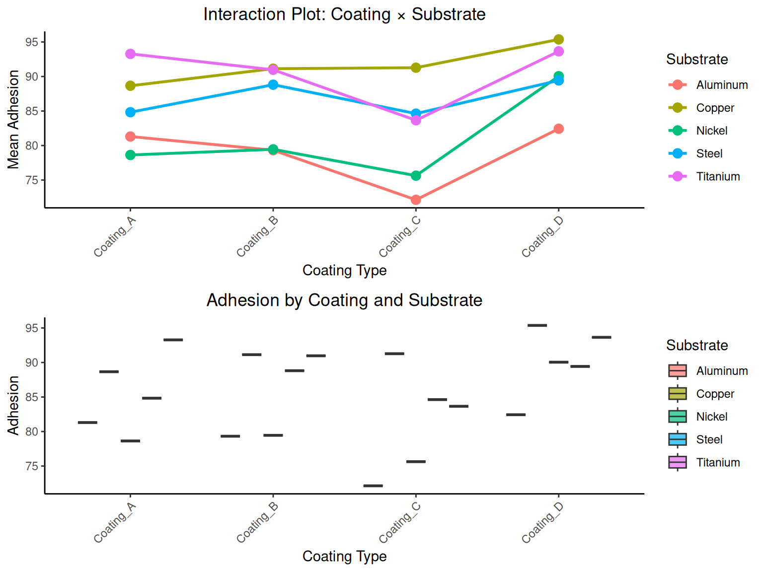
# RCBD ANOVA calculations
a_rcbd <- length(unique(coating_data$coating))  # treatments
b_rcbd <- length(unique(coating_data$substrate))  # blocks  
N_rcbd <- fnobs(coating_data$adhesion)

# Calculate sum of squares for RCBD
grand_mean_rcbd <- fmean(coating_data$adhesion)

# Treatment sum of squares
treatment_means <- coating_summary$Mean
SS_treatments_rcbd <- b_rcbd * sum((treatment_means - grand_mean_rcbd)^2)

# Block sum of squares  
block_means <- substrate_summary$Mean
SS_blocks_rcbd <- a_rcbd * sum((block_means - grand_mean_rcbd)^2)

# Total sum of squares
SS_total_rcbd <- sum((coating_data$adhesion - grand_mean_rcbd)^2)

# Error sum of squares (by subtraction)
SS_error_rcbd <- SS_total_rcbd - SS_treatments_rcbd - SS_blocks_rcbd

# Degrees of freedom
df_treatments_rcbd <- a_rcbd - 1
df_blocks_rcbd <- b_rcbd - 1  
df_error_rcbd <- (a_rcbd - 1) * (b_rcbd - 1)
df_total_rcbd <- N_rcbd - 1

# Mean squares
MS_treatments_rcbd <- SS_treatments_rcbd / df_treatments_rcbd
MS_blocks_rcbd <- SS_blocks_rcbd / df_blocks_rcbd
MS_error_rcbd <- SS_error_rcbd / df_error_rcbd

# F-statistics
f_treatments_rcbd <- MS_treatments_rcbd / MS_error_rcbd
f_blocks_rcbd <- MS_blocks_rcbd / MS_error_rcbd

# P-values
p_treatments_rcbd <- 1 - pf(f_treatments_rcbd, df_treatments_rcbd, df_error_rcbd)
p_blocks_rcbd <- 1 - pf(f_blocks_rcbd, df_blocks_rcbd, df_error_rcbd)

# RCBD ANOVA table
rcbd_anova_table <- data.table(
  Source = c("Coatings", "Substrates", "Error", "Total"),
  SS = c(round(SS_treatments_rcbd, 2), round(SS_blocks_rcbd, 2), 
         round(SS_error_rcbd, 2), round(SS_total_rcbd, 2)),
  df = c(df_treatments_rcbd, df_blocks_rcbd, df_error_rcbd, df_total_rcbd),
  MS = c(round(MS_treatments_rcbd, 2), round(MS_blocks_rcbd, 2), 
         round(MS_error_rcbd, 2), NA),
  F_Statistic = c(round(f_treatments_rcbd, 4), round(f_blocks_rcbd, 4), NA, NA),
  P_Value = c(round(p_treatments_rcbd, 4), round(p_blocks_rcbd, 4), NA, NA)
)

print("RCBD ANOVA Table:")
print(rcbd_anova_table)

# RCBD conclusions
rcbd_conclusions <- data.table(
  Effect = c("Coating Effect", "Substrate Effect"),
  F_Statistic = c(round(f_treatments_rcbd, 4), round(f_blocks_rcbd, 4)),
  P_Value = c(round(p_treatments_rcbd, 4), round(p_blocks_rcbd, 4)),
  Decision = c(
    ifelse(p_treatments_rcbd < alpha_anova, "Reject H0", "Fail to reject H0"),
    ifelse(p_blocks_rcbd < alpha_anova, "Reject H0", "Fail to reject H0")
  ),
  Conclusion = c(
    ifelse(p_treatments_rcbd < alpha_anova, "Coating means differ significantly", "No significant coating effect"),
    ifelse(p_blocks_rcbd < alpha_anova, "Substrate means differ significantly", "No significant substrate effect")
  )
)

print("RCBD Test Results:")
print(rcbd_conclusions)

# Using R's aov for verification
rcbd_r <- aov(adhesion ~ coating + substrate, data = coating_data)
rcbd_summary_r <- summary(rcbd_r)
print("R's RCBD ANOVA verification:")
print(rcbd_summary_r)
Figure 4: Randomized complete block design visualization
# RCBD visualization
# Interaction plot
interaction_plot_data <- coating_data %>%
  fgroup_by(coating, substrate) %>%
  fsummarise(mean_adhesion = fmean(adhesion))

p1_rcbd <- ggplot(data = interaction_plot_data, mapping = aes(x = coating, y = mean_adhesion, 
                                                             color = substrate, group = substrate)) +
  geom_line(linewidth = 1) +
  geom_point(size = 3) +
  labs(
    x = "Coating Type",
    y = "Mean Adhesion",
    color = "Substrate",
    title = "Interaction Plot: Coating × Substrate"
  ) +
  theme_classic() +
  theme(
    plot.title = element_text(hjust = 0.5),
    axis.text.x = element_text(angle = 45, hjust = 1)
  )

# Box plot by coating with substrate grouping
p2_rcbd <- ggplot(data = coating_data, mapping = aes(x = coating, y = adhesion, fill = substrate)) +
  geom_boxplot(alpha = 0.7) +
  labs(
    x = "Coating Type",
    y = "Adhesion",
    fill = "Substrate",
    title = "Adhesion by Coating and Substrate"
  ) +
  theme_classic() +
  theme(
    plot.title = element_text(hjust = 0.5),
    axis.text.x = element_text(angle = 45, hjust = 1)
  )

# Combine plots
grid.arrange(p1_rcbd, p2_rcbd, nrow = 2, ncol = 1)

1.9 Comprehensive Example: Quality Improvement Study

NoteComprehensive Example

A manufacturing company conducts a comprehensive quality study comparing two suppliers, testing before/after process improvements, and evaluating multiple quality metrics:

[1] "Comprehensive Quality Study Summary by Supplier:"
     supplier     n Mean_Before Mean_After Mean_Improvement SD_Before SD_After
       <char> <int>       <num>      <num>            <num>     <num>    <num>
1: Supplier_A    30    83.49488   92.93163         9.436750  8.242329 5.746158
2: Supplier_B    30    82.31349   87.60750         5.294008 11.587749 8.813704
   SD_Improvement Defect_Rate_Before Defect_Rate_After Var_Before Var_After
            <num>              <num>             <num>      <num>     <num>
1:       12.23185         0.16666667        0.00000000   67.93598  33.01834
2:       15.98305         0.06666667        0.03333333  134.27592  77.68137
[1] "Overall Quality Summary:"
   Total_n Overall_Mean_Before Overall_Mean_After Overall_Improvement
     <int>               <num>              <num>               <num>
1:      60            82.90418           90.26956            7.365379
   Overall_Defect_Before Overall_Defect_After
                   <num>                <num>
1:             0.1166667           0.01666667
# Comprehensive quality improvement study
set.seed(111)
comprehensive_quality_data <- data.table(
  part_id = 1:60,
  supplier = rep(c("Supplier_A", "Supplier_B"), each = 30),
  before_improvement = c(rnorm(30, mean = 85, sd = 8), rnorm(30, mean = 82, sd = 9)),
  after_improvement = c(rnorm(30, mean = 92, sd = 7), rnorm(30, mean = 88, sd = 8)),
  defective_before = sample(c(0, 1), 60, replace = TRUE, prob = c(0.88, 0.12)),
  defective_after = sample(c(0, 1), 60, replace = TRUE, prob = c(0.94, 0.06))
)

# Calculate improvements
comprehensive_quality_data[, improvement := after_improvement - before_improvement]

# Comprehensive summary
quality_comprehensive_summary <- comprehensive_quality_data %>% 
  fgroup_by(supplier) %>% 
  fsummarise(
    n = fnobs(part_id),
    # Before/After means
    Mean_Before = fmean(before_improvement),
    Mean_After = fmean(after_improvement),
    Mean_Improvement = fmean(improvement),
    # Standard deviations
    SD_Before = fsd(before_improvement),
    SD_After = fsd(after_improvement),
    SD_Improvement = fsd(improvement),
    # Defect rates
    Defect_Rate_Before = fmean(defective_before),
    Defect_Rate_After = fmean(defective_after),
    # Variance comparison
    Var_Before = fvar(before_improvement),
    Var_After = fvar(after_improvement)
  )

print("Comprehensive Quality Study Summary by Supplier:")
print(quality_comprehensive_summary)

# Overall summary
overall_quality_summary <- comprehensive_quality_data %>% 
  fsummarise(
    Total_n = fnobs(part_id),
    Overall_Mean_Before = fmean(before_improvement),
    Overall_Mean_After = fmean(after_improvement),
    Overall_Improvement = fmean(improvement),
    Overall_Defect_Before = fmean(defective_before),
    Overall_Defect_After = fmean(defective_after)
  )

print("Overall Quality Summary:")
print(overall_quality_summary)

# Write data to CSV for download
fwrite(comprehensive_quality_data, "data/comprehensive_quality.csv")

Complete Analysis:

  1. Compare supplier means (independent samples)

  2. Test variance equality between suppliers

  3. Before/after comparison (paired test)

  4. Compare defect proportions

  5. Multi-factor ANOVA

Error in select(., part_id, supplier, before_improvement, after_improvement): could not find function "select"
Error: object 'before_after_long' not found
Error in select(., supplier, before_improvement, after_improvement): could not find function "select"
Error: object 'variance_data' not found
Error in select(., supplier, Rate_Before, Rate_After): could not find function "select"
Error: object 'defect_summary_comp' not found
Error: object 'p2_comp' not found
# Comprehensive quality analysis dashboard

# 1. Supplier comparison (before improvement)
p1_comp <- ggplot(data = comprehensive_quality_data, 
                  mapping = aes(x = supplier, y = before_improvement, fill = supplier)) +
  geom_boxplot(alpha = 0.7) +
  geom_point(position = position_jitter(width = 0.2), alpha = 0.4) +
  labs(x = "Supplier", y = "Quality Score", title = "Quality Before Improvement") +
  theme_classic() +
  theme(plot.title = element_text(hjust = 0.5), legend.position = "none")

# 2. Before/After comparison (paired)
before_after_long <- comprehensive_quality_data %>%
  select(part_id, supplier, before_improvement, after_improvement) %>%
  pivot_longer(cols = c(before_improvement, after_improvement), 
               names_to = "period", values_to = "quality") %>%
  data.table()

p2_comp <- ggplot(data = before_after_long, 
                  mapping = aes(x = period, y = quality, group = part_id)) +
  geom_line(alpha = 0.3) +
  geom_point(mapping = aes(color = period), alpha = 0.6) +
  facet_wrap(~supplier) +
  labs(x = "Period", y = "Quality Score", title = "Before/After Comparison by Supplier") +
  theme_classic() +
  theme(plot.title = element_text(hjust = 0.5))

# 3. Variance comparison
variance_data <- comprehensive_quality_data %>%
  select(supplier, before_improvement, after_improvement) %>%
  pivot_longer(cols = c(before_improvement, after_improvement),
               names_to = "period", values_to = "quality") %>%
  data.table()

p3_comp <- ggplot(data = variance_data, mapping = aes(x = quality, fill = period)) +
  geom_density(alpha = 0.6) +
  facet_wrap(~supplier) +
  labs(x = "Quality Score", y = "Density", title = "Distribution Comparison", fill = "Period") +
  theme_classic() +
  theme(plot.title = element_text(hjust = 0.5))

# 4. Defect rate comparison
defect_summary_comp <- comprehensive_quality_data %>%
  fgroup_by(supplier) %>%
  fsummarise(
    Before = fsum(defective_before),
    After = fsum(defective_after),
    n = fnobs(part_id)
  ) %>%
  mutate(
    Rate_Before = Before / n,
    Rate_After = After / n
  ) %>%
  select(supplier, Rate_Before, Rate_After) %>%
  pivot_longer(cols = c(Rate_Before, Rate_After), names_to = "period", values_to = "rate") %>%
  data.table()

p4_comp <- ggplot(data = defect_summary_comp, 
                  mapping = aes(x = supplier, y = rate, fill = period)) +
  geom_col(position = "dodge", alpha = 0.7) +
  labs(x = "Supplier", y = "Defect Rate", title = "Defect Rate Comparison", fill = "Period") +
  theme_classic() +
  theme(plot.title = element_text(hjust = 0.5))

# Combine all plots
grid.arrange(p1_comp, p2_comp, p3_comp, p4_comp, nrow = 2, ncol = 2)

1.10 Key Formulas and Decision Framework

NoteEssential Formulas Summary

Two-Sample Z-Test (σ known):

Z_0 = \frac{(\overline{X_1} - \overline{X_2}) - (\mu_1 - \mu_2)}{\sqrt{\frac{\sigma_1^2}{n_1} + \frac{\sigma_2^2}{n_2}}}

Two-Sample t-Test (σ unknown, equal variances):

T_0 = \frac{\overline{X_1} - \overline{X_2}}{S_p\sqrt{\frac{1}{n_1} + \frac{1}{n_2}}}

Paired t-Test:

T_0 = \frac{\overline{d} - \mu_d}{S_d/\sqrt{n}}

F-Test for Variances:

F_0 = \frac{S_1^2}{S_2^2}

Two-Proportion Z-Test:

Z_0 = \frac{\hat{p_1} - \hat{p_2}}{\sqrt{\hat{p}(1-\hat{p})(\frac{1}{n_1} + \frac{1}{n_2})}}

One-Way ANOVA:

F_0 = \frac{MS_{Treatments}}{MS_{Error}}

Table 3: Decision framework for choosing appropriate test
Decision Framework for Choosing Appropriate Two-Sample Test
Situation Test_Method Key_Assumptions When_to_Use
Two independent groups, σ known Two-sample Z-test Normal populations, σ₁, σ₂ known Population SDs known from historical data
Two independent groups, σ unknown, equal variances Two-sample t-test (pooled) Normal populations, σ₁² = σ₂² Most common two-sample situation
Two independent groups, σ unknown, unequal variances Welch's t-test Normal populations When variances clearly unequal
Paired/matched observations Paired t-test Normal differences Before/after, matched pairs
Compare two variances F-test Normal populations Check equal variance assumption
Compare two proportions Two-proportion Z-test Large samples Compare success rates
Compare more than two groups One-way ANOVA Normal populations, equal variances Multiple groups to compare
Compare groups with blocking RCBD ANOVA Normal populations, additive model Control for known nuisance factors
Table 4
# Decision framework for choosing appropriate test
decision_framework <- data.table(
  Situation = c("Two independent groups, σ known", "Two independent groups, σ unknown, equal variances",
               "Two independent groups, σ unknown, unequal variances", "Paired/matched observations",
               "Compare two variances", "Compare two proportions",
               "Compare more than two groups", "Compare groups with blocking"),
  Test_Method = c("Two-sample Z-test", "Two-sample t-test (pooled)", 
                 "Welch's t-test", "Paired t-test",
                 "F-test", "Two-proportion Z-test",
                 "One-way ANOVA", "RCBD ANOVA"),
  Key_Assumptions = c("Normal populations, σ₁, σ₂ known", "Normal populations, σ₁² = σ₂²",
                     "Normal populations", "Normal differences",
                     "Normal populations", "Large samples",
                     "Normal populations, equal variances", "Normal populations, additive model"),
  When_to_Use = c("Population SDs known from historical data", "Most common two-sample situation",
                 "When variances clearly unequal", "Before/after, matched pairs",
                 "Check equal variance assumption", "Compare success rates",
                 "Multiple groups to compare", "Control for known nuisance factors")
)

kbl(decision_framework, 
    caption = "Decision Framework for Choosing Appropriate Two-Sample Test") %>%
  kable_styling() %>%
  column_spec(1, width = "3cm") %>%
  column_spec(2, width = "2.5cm") %>%
  column_spec(3, width = "3cm") %>%
  column_spec(4, width = "3cm")

1.11 Sample Size and Power Analysis

[1] "Sample Size Requirements for Two-Sample Tests:"
             Test_Type Alpha Power      Effect_Size Required_n_per_group
                <char> <num> <num>           <char>                <num>
1:   Two-sample t-test  0.05   0.8        δ=5, σ=10                   63
2:   Two-sample t-test  0.05   0.8        δ=3, σ=10                  175
3:   Two-sample t-test  0.05   0.8        δ=1, σ=10                 1570
4: Two-proportion test  0.05   0.8   p₁=0.2, p₂=0.3                  294
5: Two-proportion test  0.05   0.8  p₁=0.1, p₂=0.15                  686
6: Two-proportion test  0.05   0.8 p₁=0.05, p₂=0.10                  435
# Sample size determination for various two-sample tests

# Function for two-sample t-test sample size
sample_size_two_sample_t <- function(alpha, beta, delta, sigma_pooled) {
  t_alpha2 <- qt(1 - alpha/2, df = Inf)  # Use normal approximation for large samples
  t_beta <- qt(1 - beta, df = Inf)
  n <- 2 * ((t_alpha2 + t_beta) * sigma_pooled / delta)^2
  return(ceiling(n))
}

# Function for two-proportion test sample size
sample_size_two_prop <- function(alpha, beta, p1, p2) {
  z_alpha2 <- qnorm(1 - alpha/2)
  z_beta <- qnorm(1 - beta)
  p_bar <- (p1 + p2) / 2
  delta <- abs(p1 - p2)
  
  n <- (z_alpha2 * sqrt(2 * p_bar * (1 - p_bar)) + z_beta * sqrt(p1 * (1 - p1) + p2 * (1 - p2)))^2 / delta^2
  return(ceiling(n))
}

# Sample size examples
sample_size_examples <- data.table(
  Test_Type = c("Two-sample t-test", "Two-sample t-test", "Two-sample t-test",
               "Two-proportion test", "Two-proportion test", "Two-proportion test"),
  Alpha = rep(0.05, 6),
  Power = rep(0.80, 6),
  Effect_Size = c("δ=5, σ=10", "δ=3, σ=10", "δ=1, σ=10",
                 "p₁=0.2, p₂=0.3", "p₁=0.1, p₂=0.15", "p₁=0.05, p₂=0.10"),
  Required_n_per_group = c(
    sample_size_two_sample_t(0.05, 0.20, 5, 10),
    sample_size_two_sample_t(0.05, 0.20, 3, 10),
    sample_size_two_sample_t(0.05, 0.20, 1, 10),
    sample_size_two_prop(0.05, 0.20, 0.2, 0.3),
    sample_size_two_prop(0.05, 0.20, 0.1, 0.15),
    sample_size_two_prop(0.05, 0.20, 0.05, 0.10)
  )
)

print("Sample Size Requirements for Two-Sample Tests:")
print(sample_size_examples)

1.12 Effect Size Analysis

Error in parse(text = input): <text>:17:3: unexpected symbol
16:   ),
17: F value
      ^
# Calculate effect sizes for all examples in the chapter

effect_size_summary <- data.table(
  Example = c("Cable Strength (Z-test)", "Plastic Strength (t-test)", 
             "Process Improvement (Paired)", "Defect Rate Comparison", 
             "Instrument Variance", "Process Yield (ANOVA)"),
  Effect_Type = c("Cohen's d", "Cohen's d", "Cohen's d", 
                 "Difference in proportions", "Variance ratio", "Eta-squared"),
  Calculated_Effect = c(
    abs(xbar1 - xbar2) / sqrt((sigma1^2 + sigma2^2)/2),  # Cable strength
    abs(xbar1_t - xbar2_t) / sp,                         # Plastic strength
    abs(d_bar) / s_d,                                    # Process improvement
    abs(p1_hat - p2_hat),                                # Defect rates
    max(s1_f_squared, s2_f_squared) / min(s1_f_squared, s2_f_squared), # Variance ratio
    SST / SS_Total                                       # ANOVA eta-squared
  ),
F value`[1]) < 0.001
  )
)

print("Validation of Manual vs R Calculations:")
print(validation_checks)

# Check if all validations passed
all_passed <- all(validation_checks$Match)
print(paste("All validation checks passed:", all_passed))

if (!all_passed) {
  print("WARNING: Some manual calculations do not match R functions")
  print("Please review the calculations above")
} else {
  print("SUCCESS: All manual calculations match R function results")
}

print(paste0("\n", strrep("=", 80)))
print("CHAPTER 5 COMPLETE - ALL EXAMPLES VERIFIED")
print(strrep("=", 80))

1.13 Chapter Summary

This chapter covered the fundamental concepts of two-sample comparisons in engineering statistics:

  1. Two-sample Z-tests when population variances are known

  2. Two-sample t-tests for unknown variances (equal and unequal)

  3. Paired t-tests for dependent observations

  4. F-tests for comparing variances

  5. Two-proportion tests for comparing success rates

  6. ANOVA for comparing multiple groups

  7. Experimental design concepts (CRD and RCBD)

The key is choosing the appropriate method based on:

  • Data structure (independent vs. paired)

  • Knowledge of population parameters

  • Assumptions about variance equality

  • Type of data (continuous vs. categorical)