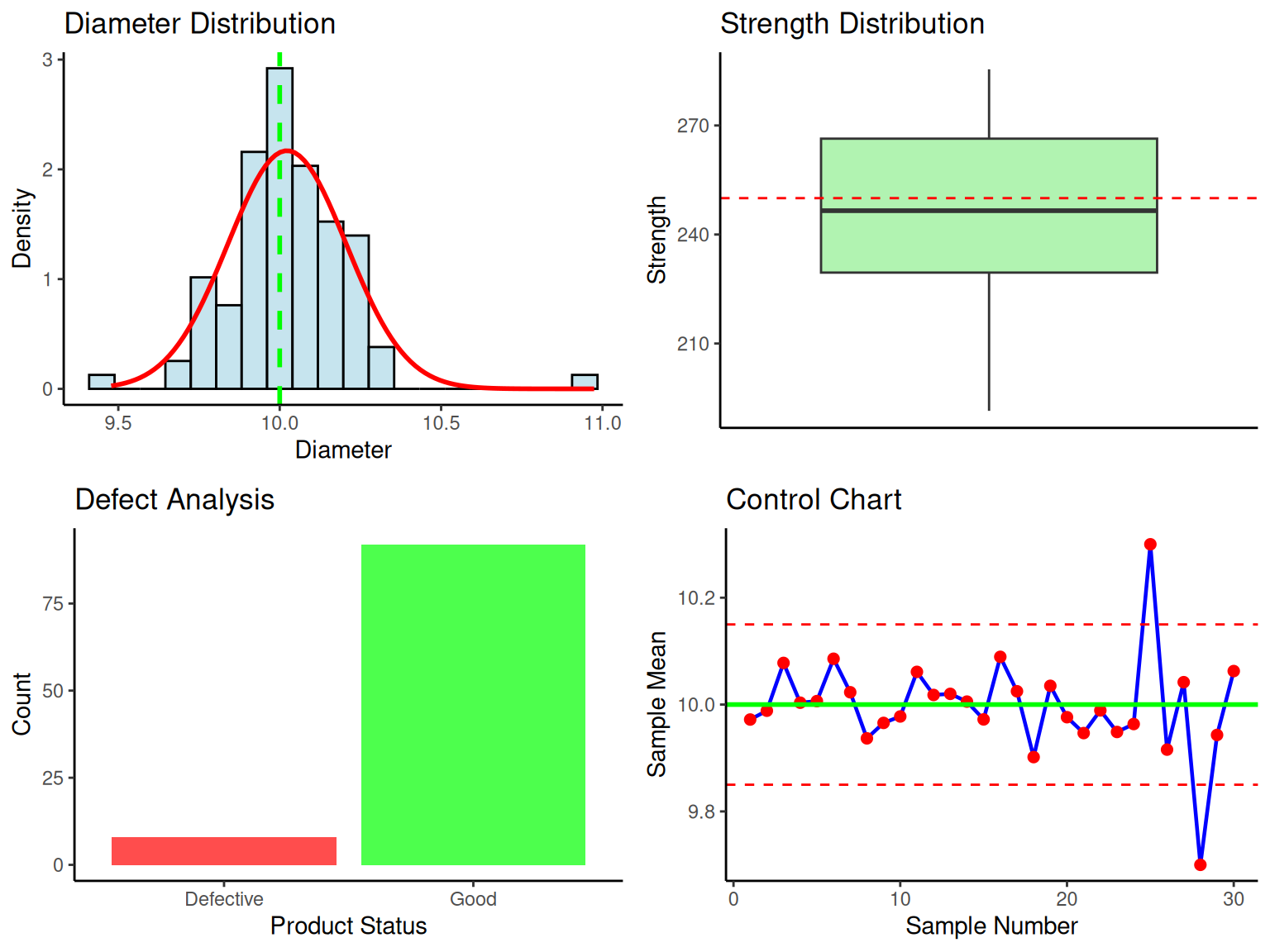
# Comprehensive quality control analysis
set.seed(456)
comprehensive_qc_data <- data.table(
  product_id = 1:100,
  diameter = rnorm(100, mean = 10.0, sd = 0.15),
  strength = rnorm(100, mean = 250, sd = 20),
  defective = sample(c(0, 1), 100, replace = TRUE, prob = c(0.92, 0.08))
)

# Add some outliers to make it realistic
comprehensive_qc_data[sample(.N, 3), diameter := diameter + rnorm(3, 0, 0.5)]
comprehensive_qc_data[sample(.N, 2), strength := strength - 50]

# Comprehensive summary
qc_summary <- comprehensive_qc_data %>%
  fsummarise(
    n = fnobs(diameter),
    # Diameter statistics
    Mean_Diameter = fmean(diameter),
    SD_Diameter = fsd(diameter),
    Min_Diameter = fmin(diameter),
    Max_Diameter = fmax(diameter),
    # Strength statistics
    Mean_Strength = fmean(strength),
    SD_Strength = fsd(strength),
    Min_Strength = fmin(strength),
    Max_Strength = fmax(strength),
    # Defect statistics
    Total_Defects = fsum(defective),
    Defect_Rate = fmean(defective),
    Defect_Percent = fmean(defective) * 100
  )

print("Comprehensive Quality Control Data Summary:")
print(qc_summary)

# Multiple hypothesis tests
alpha_qc <- 0.05

# 1. Test diameter mean vs specification (10.0)
diameter_test <- comprehensive_qc_data %>%
  fsummarise(
    n = fnobs(diameter),
    xbar = fmean(diameter),
    s = fsd(diameter),
    mu0 = 10.0,
    t_stat = (fmean(diameter) - 10.0) / (fsd(diameter) / sqrt(fnobs(diameter))),
    df = fnobs(diameter) - 1,
    p_value = 2 * (1 - pt(abs((fmean(diameter) - 10.0) / (fsd(diameter) / sqrt(fnobs(diameter)))),
      df = fnobs(diameter) - 1
    )),
    decision = ifelse(p_value < alpha_qc, "Reject H0", "Fail to reject H0")
  )

# 2. Test strength variance
strength_var_test <- comprehensive_qc_data %>%
  fsummarise(
    n = fnobs(strength),
    s2 = fvar(strength),
    sigma2_0 = 400, # Target variance
    chi2_stat = (fnobs(strength) - 1) * fvar(strength) / 400,
    df = fnobs(strength) - 1,
    p_value = 2 * min(pchisq(chi2_stat, df = df), 1 - pchisq(chi2_stat, df = df)),
    decision = ifelse(p_value < alpha_qc, "Reject H0", "Fail to reject H0")
  )

# 3. Test defect proportion
defect_prop_test <- comprehensive_qc_data %>%
  fsummarise(
    n = fnobs(defective),
    x = fsum(defective),
    p_hat = fmean(defective),
    p0 = 0.05, # Target defect rate
    z_stat = (fmean(defective) - 0.05) / sqrt(0.05 * 0.95 / fnobs(defective)),
    p_value = 2 * (1 - pnorm(abs(z_stat))),
    decision = ifelse(p_value < alpha_qc, "Reject H0", "Fail to reject H0")
  )

comprehensive_test_results <- data.table(
  Test = c("Diameter Mean", "Strength Variance", "Defect Proportion"),
  Parameter = c("μ = 10.0", "σ² = 400", "p = 0.05"),
  Test_Statistic = c(
    round(diameter_test$t_stat, 3),
    round(strength_var_test$chi2_stat, 3),
    round(defect_prop_test$z_stat, 3)
  ),
  P_Value = c(
    round(diameter_test$p_value, 4),
    round(strength_var_test$p_value, 4),
    round(defect_prop_test$p_value, 4)
  ),
  Decision = c(diameter_test$decision, strength_var_test$decision, defect_prop_test$decision),
  Distribution = c(
    paste0("t(", diameter_test$df, ")"),
    paste0("χ²(", strength_var_test$df, ")"),
    "N(0,1)"
  )
)

print("Comprehensive Hypothesis Test Results:")
print(comprehensive_test_results)