Partial diallel analysis (crosses between two groups of parents)

PartialDiallel() analyses a partial diallel in which each of $L$ parents of a first group is crossed with each of $M$ parents of a second group (a factorial mating design, also known as line by tester or North Carolina design II), from the plot data of a randomized complete block experiment: the analysis of variance of the general combining ability of each group and of the specific combining ability, the variance components, and the gca and sca effects.

Usage

PartialDiallel(y, Rep, Cross1, Cross2, data)

Arguments

y: response: a column of data given by name (y = Yield or y = "Yield") or a numeric vector of length nrow(data).
Rep: replicate (block): a column of data or a vector, as for y.
Cross1: parent of group I (rows) of each plot: a column of data or a vector, as for y.
Cross2: parent of group II (columns) of each plot: a column of data or a vector, as for y.
data: a data frame (or data.table) with one row per plot.

Value

An object of class c("da_partial", "da_result", "list"):

Means: $L \times M$ matrix of cross means.
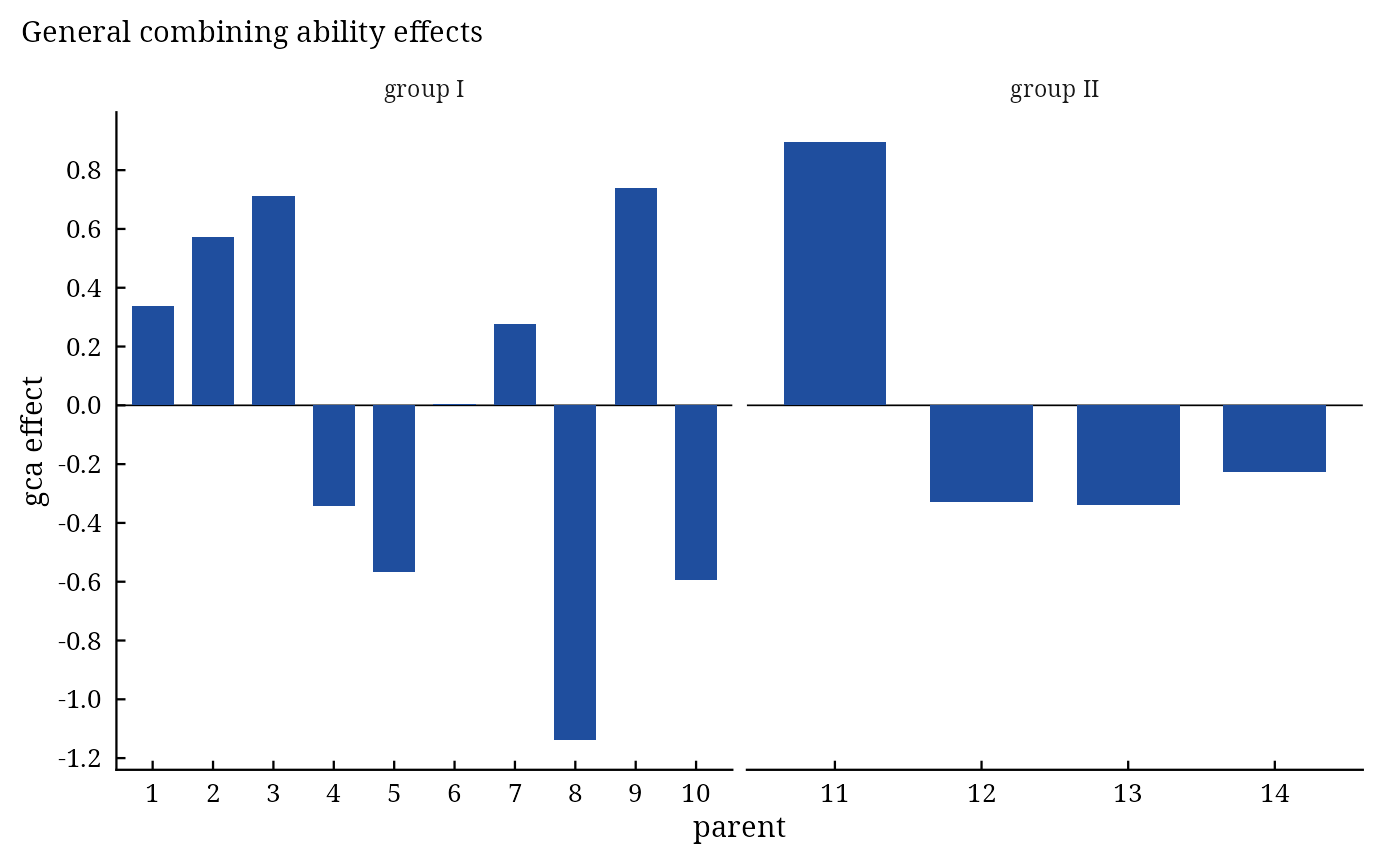
ANOVA: analysis of variance (class anova): Treat, GCA I, GCA II, SCA, Error.
Genetic.Components: Components (variance components of GCA I, GCA II, SCA) and Percent (share of the treatment sum of squares, as a proportion).
General: gca effects, group I followed by group II, named by parent.
Specific: $L \times M$ matrix of sca effects.
RCBD: (new) analysis of variance of the plot data as a randomized complete block design.

Methods: print(), summary(), plot() (gca effects of both groups and the sca effects as a heat map, residual plots; which = c("gca", "sca", "residuals", "qq")), anova(), coef(), vcov(), confint(), fitted(), residuals(), data.table::as.data.table(x, component =); see diallel-methods.

Details

Data and model. $\mathbf{Y}$ is the $L \times M$ matrix of cross means (group I in rows, group II in columns) over $B$ replicates, with row means $\bar{Y}_{i\cdot}$, column means $\bar{Y}_{\cdot j}$ and grand mean $\bar{Y}_{\cdot\cdot}$. The mean of cross $i \times j$ is $Y_{ij} = \mu + g^{I}_i + g^{II}_j + S_{ij} + \bar{e}_{ij}$.

Analysis of variance (plot scale): $$SS_{g^I} = BM\sum_i (\bar{Y}_{i\cdot} - \bar{Y}_{\cdot\cdot})^2, \quad SS_{g^{II}} = BL\sum_j (\bar{Y}_{\cdot j} - \bar{Y}_{\cdot\cdot})^2, \quad SS_s = B\sum_{i,j}(Y_{ij} - \bar{Y}_{i\cdot} - \bar{Y}_{\cdot j} + \bar{Y}_{\cdot\cdot})^2,$$ on $L-1$, $M-1$ and $(L-1)(M-1)$ degrees of freedom; their sum is the treatment sum of squares on $LM-1$ degrees of freedom; the error is the residual of the block analysis of the plot data. Every line is tested against the error.

Effects. $\hat{g}^I_i = \bar{Y}_{i\cdot} - \bar{Y}_{\cdot\cdot}$, $\hat{g}^{II}_j = \bar{Y}_{\cdot j} - \bar{Y}_{\cdot\cdot}$, $\hat{S}_{ij} = Y_{ij} - \bar{Y}_{i\cdot} - \bar{Y}_{\cdot j} + \bar{Y}_{\cdot\cdot}$.

Variance components (random model; Kempthorne 1957, Comstock and Robinson 1952): $\sigma^2_{g^I} = (MS_{g^I} - MS_s)/(BM)$, $\sigma^2_{g^{II}} = (MS_{g^{II}} - MS_s)/(BL)$, $\sigma^2_s = (MS_s - MS_E)/B$. The column Percent gives the proportional contribution of each source to the treatment sum of squares.

Changes from version 0.6.0. The column arguments are used (version 0.6.0 read the columns y, Rep, Cross1 and Cross2 by name); the error line is on the plot scale like the other lines (version 0.6.0 divided it by the number of replicates, so its $F$ values were too large by that factor squared); the components are the variance components above (version 0.6.0 gave differences of mean squares and their shares); the tables keep the parents' labels.

References

Comstock, R. E. and Robinson, H. F. (1952). Estimation of average dominance of genes. In J. W. Gowen (ed.), Heterosis, 494–516. Iowa State College Press, Ames.

Kempthorne, O. (1957). An Introduction to Genetic Statistics. John Wiley and Sons, New York.

Kempthorne, O. and Curnow, R. N. (1961). The partial diallel cross. Biometrics, 17(2), 229–250. doi:10.2307/2527989

Singh, R. K. and Chaudhary, B. D. (2004). Biometrical Methods in Quantitative Genetic Analysis. Kalyani Publishers, New Delhi.

Author

Muhammad Yaseen (myaseen208@gmail.com), Pedro A. M. Barbosa (pedro.barbosa@usp.br)

Examples

#-------------------------------------------------------------
## Ten parents of group I crossed with four parents of group II
#-------------------------------------------------------------
Partial1 <-
  PartialDiallel(
      y      = y
    , Rep    = Rep
    , Cross1 = Cross1
    , Cross2 = Cross2
    , data   = PartialDiallelData
    )
Partial1
#> Partial diallel; 10 x 4 parents 
#> 
#> Analysis of variance
#>         Df Sum Sq Mean Sq F value   Pr(>F)    
#> Treat   39 144.77   3.712   2.746 1.56e-05 ***
#> GCA I    9  58.54   6.505   4.812 1.81e-05 ***
#> GCA II   3  43.05  14.351  10.616 3.16e-06 ***
#> SCA     27  43.18   1.599   1.183    0.265    
#> Error  117 158.17   1.352                     
#> ---
#> Signif. codes:  0 ‘***’ 0.001 ‘**’ 0.01 ‘*’ 0.05 ‘.’ 0.1 ‘ ’ 1
#> 
#> Variance components
#>        Components Percent
#> GCA I     0.30659  0.4044
#> GCA II    0.31879  0.2974
#> SCA       0.06185  0.2983
#> 
#> General combining ability effects
#>       1       2       3       4       5       6       7       8       9      10 
#>  0.3381  0.5712  0.7119 -0.3425 -0.5669  0.0050  0.2750 -1.1380  0.7406 -0.5944 
#>      11      12      13      14 
#>  0.8953 -0.3293 -0.3390 -0.2270 
#> 
#> All components: names(x); tests of the effects: summary(x); figures: plot(x)
Partial1$ANOVA
#>         Df  Sum Sq Mean Sq F value    Pr(>F)    
#> Treat   39 144.775  3.7122  2.7460 1.559e-05 ***
#> GCA I    9  58.542  6.5046  4.8116 1.810e-05 ***
#> GCA II   3  43.053 14.3510 10.6158 3.165e-06 ***
#> SCA     27  43.180  1.5993  1.1830    0.2654    
#> Error  117 158.167  1.3519                      
#> ---
#> Signif. codes:  0 ‘***’ 0.001 ‘**’ 0.01 ‘*’ 0.05 ‘.’ 0.1 ‘ ’ 1
Partial1$Genetic.Components
#>        Components   Percent
#> GCA I  0.30658640 0.4043642
#> GCA II 0.31879459 0.2973799
#> SCA    0.06185035 0.2982560
plot(Partial1)