Line by tester analysis

LineTester() carries out Kempthorne's (1957) line $\times$ tester analysis of the crosses of $L$ lines with $T$ testers in a randomized complete block experiment: the analysis of variance with the split of the crosses into lines, testers and lines $\times$ testers, the proportional contributions of the three to the crosses' sum of squares, the general and specific combining ability effects with standard errors, and the genetic variances.

Usage

LineTester(y, Rep, Line, Tester, data, Inbreeding = 0)

Arguments

y: response: a column of data given by name (y = Yield or y = "Yield") or a numeric vector of length nrow(data).
Rep: replicate (block): a column of data or a vector, as for y.
Line: line (female) of each plot: a column of data or a vector, as for y.
Tester: tester (male) of each plot: a column of data or a vector, as for y.
data: a data frame (or data.table) with one row per plot.
Inbreeding: inbreeding coefficient $F$ of the lines and testers, in $[0, 1]$ (default 0; 1 for inbred lines).

Value

An object of class c("da_linetester", "da_result", "list"):

Means: $L \times T$ matrix of cross means.
ANOVA: analysis of variance (class anova): Rep, Crosses, Lines, Testers, Lines:Testers, Error.
Contribution: proportional contributions (percent) of lines, testers and lines $\times$ testers.
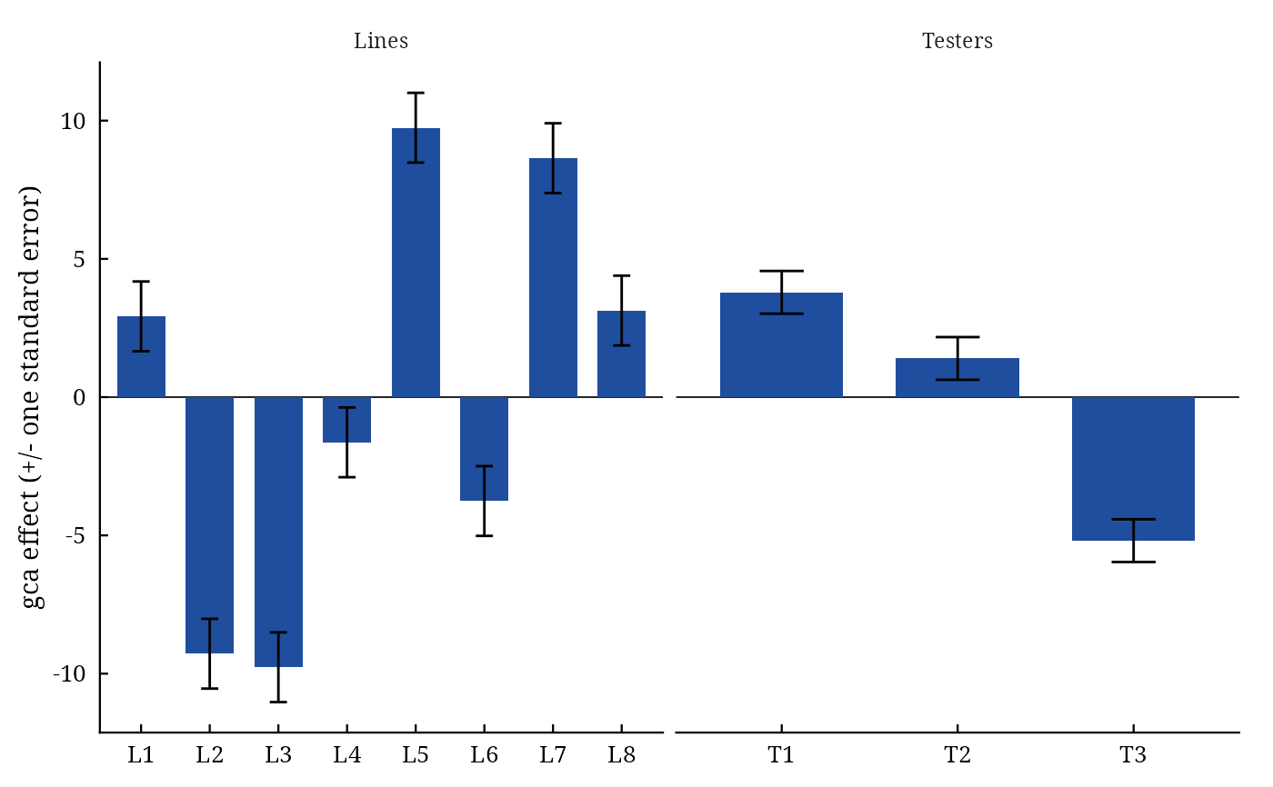
GCA.Lines, GCA.Testers: gca effects (named vectors).
SCA: $L \times T$ matrix of sca effects.
StdErr: standard errors: gca_line, gca_tester, sca, gi_gj_line, gi_gj_tester, sij_skl.
Genetic.Components: data frame: $\sigma^2_{gca}$ of lines, of testers and pooled, $\sigma^2_{sca}$, $\sigma^2_A$, $\sigma^2_D$, their ratio and the degree of dominance.

Methods: print(), summary(), plot() (which = c("gca", "sca", "contribution", "biplot", "residuals", "qq")), data.table::as.data.table(x, component =), da_export.

Details

With $B$ replicates, cross means $\bar{y}_{ij}$, line means $\bar{y}_{i\cdot}$, tester means $\bar{y}_{\cdot j}$ and grand mean $\bar{y}_{\cdot\cdot}$: $$\hat{g}_i = \bar{y}_{i\cdot} - \bar{y}_{\cdot\cdot}, \quad \hat{g}_j = \bar{y}_{\cdot j} - \bar{y}_{\cdot\cdot}, \quad \hat{s}_{ij} = \bar{y}_{ij} - \bar{y}_{i\cdot} - \bar{y}_{\cdot j} + \bar{y}_{\cdot\cdot},$$ with standard errors $\sqrt{MS_E/(BT)}$ (lines), $\sqrt{MS_E/(BL)}$ (testers) and $\sqrt{MS_E/B}$ (crosses); a difference of two effects has $\sqrt{2}$ times these. The sums of squares are on the plot scale; the proportional contribution of lines is $100 SS_L/SS_C$, and likewise for testers and lines $\times$ testers.

Genetic variances. From the expected mean squares $E(MS_L) = \sigma^2 + B\sigma^2_s + BT\sigma^2_{gL}$, $E(MS_T) = \sigma^2 + B\sigma^2_s + BL\sigma^2_{gT}$ and $E(MS_{LT}) = \sigma^2 + B\sigma^2_s$: $$\hat{\sigma}^2_{gca} = \frac{L + T - 2}{B(2LT - L - T)}\left[\frac{(L - 1)MS_L + (T - 1)MS_T}{L + T - 2} - MS_{LT}\right], \qquad \hat{\sigma}^2_{sca} = \frac{MS_{LT} - MS_E}{B},$$ and with inbreeding coefficient $F$ of the parents $\sigma^2_A = 4\sigma^2_{gca}/(1 + F)$ and $\sigma^2_D = 4\sigma^2_{sca}/(1 + F)^2$ (Singh and Chaudhary 2004). The degree of dominance is $\sqrt{2\sigma^2_D/\sigma^2_A}$.

Missing plots are handled as in Griffing: least-squares cross means adjusted for blocks and the harmonic mean of the plot numbers as $B$; every cross must have at least one plot.

References

Kempthorne, O. (1957). An Introduction to Genetic Statistics. John Wiley and Sons, New York.

Singh, R. K. and Chaudhary, B. D. (2004). Biometrical Methods in Quantitative Genetic Analysis. Kalyani Publishers, New Delhi.

Author

Muhammad Yaseen (myaseen208@gmail.com)

Examples

lt <-
  LineTester(
      y          = Yield
    , Rep        = Rep
    , Line       = Line
    , Tester     = Tester
    , data       = LineTesterData
    , Inbreeding = 1
    )
lt
#> Line x tester analysis: 8 lines, 3 testers, 3 replicates 
#> 
#>               Df Sum Sq Mean Sq F value   Pr(>F)    
#> Rep            2    427   213.3  14.894 1.03e-05 ***
#> Crosses       23   5469   237.8  16.607 2.76e-15 ***
#> Lines          7   3476   496.6  34.685 2.70e-16 ***
#> Testers        2   1038   519.0  36.244 3.54e-10 ***
#> Lines:Testers 14    955    68.2   4.762 2.76e-05 ***
#> Error         46    659    14.3                     
#> ---
#> Signif. codes:  0 ‘***’ 0.001 ‘**’ 0.01 ‘*’ 0.05 ‘.’ 0.1 ‘ ’ 1
#> 
#> Proportional contributions (%)
#>         Lines       Testers Lines:Testers 
#>         63.57         18.98         17.45 
#> 
#> Genetic components
#>                     Components
#> gca_lines              47.6060
#> gca_testers            18.7824
#> gca                    35.1418
#> sca                    17.9554
#> gca/sca                 1.9572
#> Additive               70.2835
#> Dominance              17.9554
#> Dominance/Additive      0.2555
#> Degree of dominance     0.7148
lt$Contribution
#>         Lines       Testers Lines:Testers 
#>      63.56706      18.97840      17.45454 
plot(x = lt, which = c("gca", "sca", "contribution", "biplot", "residuals", "qq")[1])