Gardner and Eberhart's Analyses II and III of a diallel with parents

GardnerEberhart() analyses parents and one set of $F_1$ crosses (Griffing's Method 2 design) with the genetic models of Gardner and Eberhart (1966): Analysis II splits the entries into variety effects and heterosis (average, variety and specific heterosis); Analysis III into variety effects, average heterosis and the general and specific combining ability of the crosses.

Usage

GardnerEberhart(y, Rep, Cross1, Cross2, data, Analysis = 2, Model = 1)

Arguments

y: response: a column of data given by name (y = Yield or y = "Yield") or a numeric vector of length nrow(data).
Rep: replicate (block): a column of data or a vector, as for y.
Cross1: female parent of each plot: a column of data or a vector, as for y.
Cross2: male parent of each plot: a column of data or a vector, as for y.
data: a data frame (or data.table) with one row per plot.
Analysis: 2 (Analysis II, default) or 3 (Analysis III).
Model: 1 (fixed effects, default) or 2 (random effects; changes only the tests).

Value

An object of class c("da_gardner", "da_result", "list"):

Means: matrix of entry means (parents on the diagonal, crosses above it).
ANOVA: analysis of variance of the entries (class anova).
Effects: data.table of the effects of each parent with standard errors: Analysis II v and h; Analysis III v and g.
Average: data frame: $\hat{\mu}_v$ and $\hat{\bar{h}}$ with standard errors.
Specific: symmetric matrix of the specific effects $\hat{s}_{jj'}$.
RCBD: analysis of variance of the plot data.

Methods: print(), summary(), plot() (which = c("effects", "specific", "residuals", "qq")), data.table::as.data.table(x, component =), da_export.

Details

Let $\bar{y}_{jj}$ be the mean of parent (variety) $j$ and $\bar{y}_{jj'}$ that of the cross $j \times j'$, $j < j'$, with $P$ parents.

Analysis II. $$\bar{y}_{jj} = \mu_v + v_j, \qquad \bar{y}_{jj'} = \mu_v + \frac{v_j + v_{j'}}{2} + \bar{h} + h_j + h_{j'} + s_{jj'},$$ with $\sum_j v_j = \sum_j h_j = 0$ and $\sum_{j' \neq j} s_{jj'} = 0$. The entries' sum of squares ($P(P + 1)/2 - 1$ degrees of freedom) is split sequentially into varieties ($P - 1$) and heterosis, the latter into average heterosis (1), variety heterosis ($P - 1$) and specific heterosis ($P(P - 3)/2$).

Analysis III. $$\bar{y}_{jj} = \mu_v + v_j, \qquad \bar{y}_{jj'} = \mu_v + \bar{h} + g_j + g_{j'} + s_{jj'},$$ with $\sum_j g_j = 0$: varieties ($P - 1$), varieties against crosses (average heterosis, 1), general combining ability of the crosses ($P - 1$) and specific combining ability ($P(P - 3)/2$); the last two are Griffing's Method 4 analysis of the crosses.

The sums of squares are on the scale of entry means; the error is $MS_E/B$ on the error degrees of freedom of the block analysis (least-squares entry means and the harmonic mean of the plot numbers when plots are missing). With Model = 1 every line is tested against the error; with Model = 2 the variety and heterosis lines (Analysis II) or the gca line (Analysis III) are tested against the specific line. Standard errors of the effects come from the least-squares fit, $\mathrm{Var}(\hat{\boldsymbol{\beta}}) = (\mathbf{X}^{\top}\mathbf{X})^{-1}MS_E/B$.

References

Gardner, C. O. and Eberhart, S. A. (1966). Analysis and interpretation of the variety cross diallel and related populations. Biometrics, 22(3), 439–452. doi:10.2307/2528181

Murray, L. W., Ray, I. M., Dong, H. and Segovia-Lerma, A. (2003). Clarification and reevaluation of population-based diallel analyses: Gardner and Eberhart Analyses II and III revisited. Crop Science, 43(6), 1930–1937. doi:10.2135/cropsci2003.1930

Author

Muhammad Yaseen (myaseen208@gmail.com)

Examples

#-------------------------------------------------------------
## Analysis II: varieties and heterosis
#-------------------------------------------------------------
ge2 <-
  GardnerEberhart(
      y        = Yield
    , Rep      = Rep
    , Cross1   = Cross1
    , Cross2   = Cross2
    , data     = GriffingData2
    , Analysis = 2
    , Model    = 1
    )
ge2
#> Gardner and Eberhart's Analysis II, Model 1; 8 parents, 4 replicates 
#> 
#> Analysis of variance (entry means)
#>                     Df Sum Sq Mean Sq F value   Pr(>F)    
#> Varieties            7   1851   264.4    9.47 4.55e-09 ***
#> Heterosis           28  12529   447.5   16.03  < 2e-16 ***
#> Average heterosis    1    374   373.8   13.39 0.000398 ***
#> Variety heterosis    7   2851   407.2   14.59 3.81e-13 ***
#> Specific heterosis  20   9305   465.2   16.66  < 2e-16 ***
#> Error              105   2932    27.9                     
#> ---
#> Signif. codes:  0 ‘***’ 0.001 ‘**’ 0.01 ‘*’ 0.05 ‘.’ 0.1 ‘ ’ 1
#> 
#>      Estimate Std. Error t value  Pr(>|t|)
#> mu_v   84.633      1.868  45.302 9.626e-71
#> hbar    7.751      2.118   3.659 3.980e-04
#> 
#> Effects of the parents
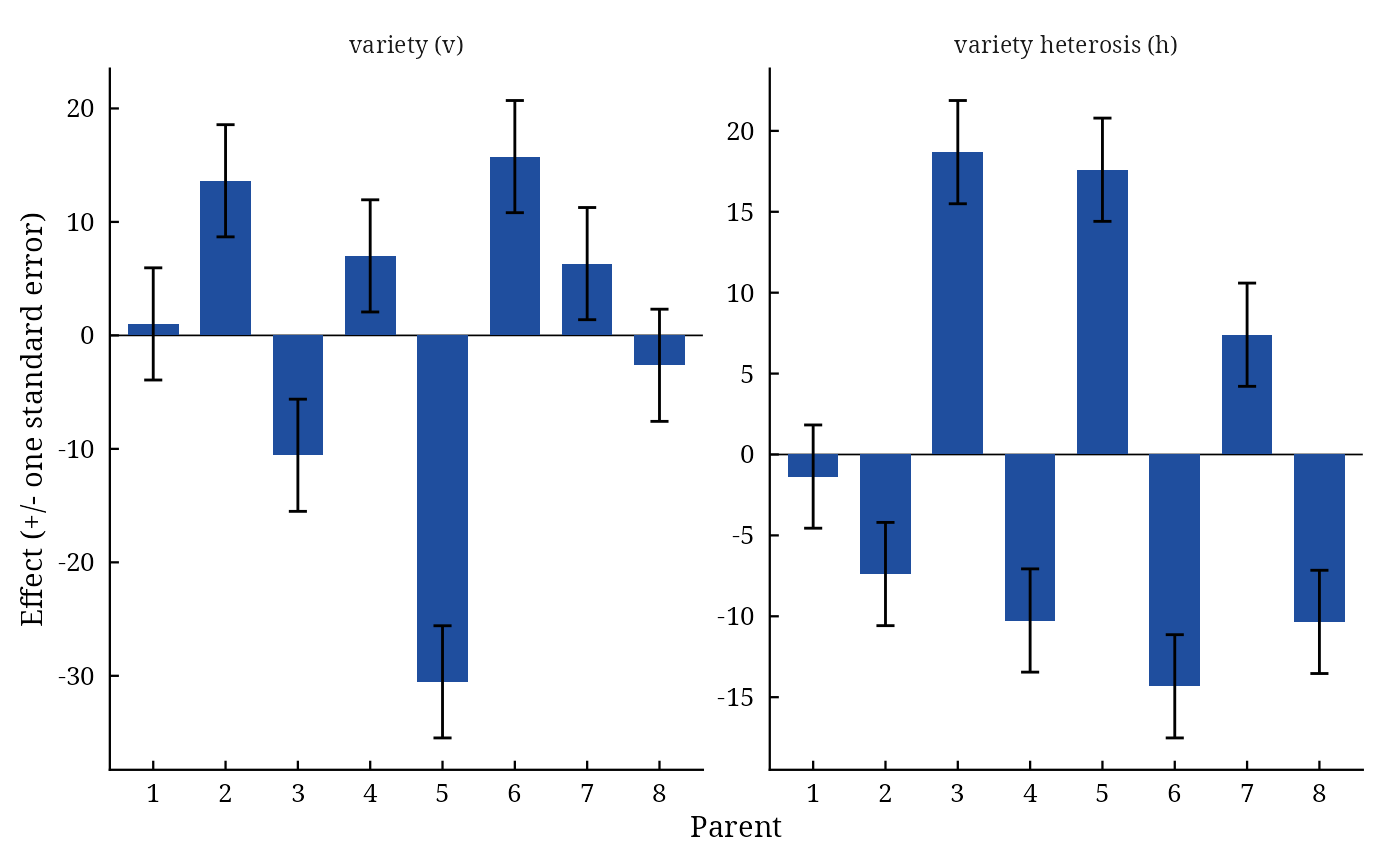
#>    Parent       v  SE_v       h  SE_h
#>    <char>   <num> <num>   <num> <num>
#> 1:      1   1.012 4.943  -1.365 3.191
#> 2:      2  13.627 4.943  -7.388 3.191
#> 3:      3 -10.563 4.943  18.687 3.191
#> 4:      4   7.007 4.943 -10.261 3.191
#> 5:      5 -30.531 4.943  17.600 3.191
#> 6:      6  15.757 4.943 -14.328 3.191
#> 7:      7   6.327 4.943   7.403 3.191
#> 8:      8  -2.633 4.943 -10.347 3.191
ge2$Effects
#>    Parent          v     SE_v          h     SE_h
#>    <char>      <num>    <num>      <num>    <num>
#> 1:      1   1.011562 4.942814  -1.365469 3.190573
#> 2:      2  13.626563 4.942814  -7.388385 3.190573
#> 3:      3 -10.563438 4.942814  18.686615 3.190573
#> 4:      4   7.006563 4.942814 -10.260885 3.190573
#> 5:      5 -30.530938 4.942814  17.599531 3.190573
#> 6:      6  15.756562 4.942814 -14.327552 3.190573
#> 7:      7   6.326563 4.942814   7.402865 3.190573
#> 8:      8  -2.633437 4.942814 -10.346719 3.190573
plot(x = ge2, which = c("effects", "specific", "residuals", "qq")[1])


#-------------------------------------------------------------
## Analysis III: varieties, average heterosis, gca and sca
#-------------------------------------------------------------
ge3 <-
  GardnerEberhart(
      y        = Yield
    , Rep      = Rep
    , Cross1   = Cross1
    , Cross2   = Cross2
    , data     = GriffingData2
    , Analysis = 3
    , Model    = 1
    )
ge3$ANOVA
#>                    Df Sum Sq Mean Sq F value    Pr(>F)    
#> Varieties           7 1574.8  224.96   8.057 8.099e-08 ***
#> Average heterosis   1  373.8  373.81  13.388  0.000398 ***
#> gca                 7 3126.9  446.70  15.998 3.672e-14 ***
#> sca                20 9304.6  465.23  16.662 < 2.2e-16 ***
#> Error             105 2931.8   27.92                      
#> ---
#> Signif. codes:  0 ‘***’ 0.001 ‘**’ 0.01 ‘*’ 0.05 ‘.’ 0.1 ‘ ’ 1