Griffing's diallel analysis over several environments

GriffingEnv() combines Griffing's analysis of the same diallel grown in several environments (locations, years or seasons), each a randomized complete block experiment: the pooled analysis of variance with the interactions gca $\times$ environment, sca $\times$ environment and, in Methods 1 and 3, reciprocal $\times$ environment, the effects from the means over environments, the gca effects in every environment and, in the random model, the variance components.

Usage

GriffingEnv(y, Rep, Cross1, Cross2, Env, data, Method, Model)

Arguments

y: response: a column of data given by name (y = Yield or y = "Yield") or a numeric vector of length nrow(data).
Rep: replicate (block): a column of data or a vector, as for y.
Cross1: female parent of each plot: a column of data or a vector, as for y.
Cross2: male parent of each plot: a column of data or a vector, as for y.
Env: environment of each plot: a column of data or a vector, as for y. Replicate labels are taken within environments.
data: a data frame (or data.table) with one row per plot.
Method: 1 (parents, $F_1$ and reciprocals), 2 (parents and one set of $F_1$), 3 ($F_1$ and reciprocals) or 4 (one set of $F_1$). No default.
Model: 1 (fixed effects) or 2 (random effects). No default.

Value

An object of class c("da_griffingenv", "da_result", "list"):

Means: table of cross means over environments.
ANOVA: pooled analysis of variance (class anova).
GCA: gca effects over environments; GCA.Env: matrix of gca effects, parents by environments.
SCA: sca effects over environments; Reciprocal (Methods 1 and 3) reciprocal effects.
StdErr: standard errors of the effects over environments, as in Griffing.
Genetic.Components: (Model 2) variance components.
ByEnv: list of the single-environment Griffing analyses.

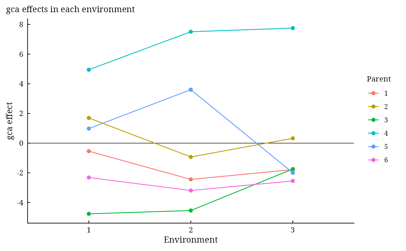
Methods: print(), summary(), plot() (which = c("gca", "gcaenv", "sca", "residuals", "qq"); "gcaenv" draws the gca effect of every parent in every environment), data.table::as.data.table(x, component =), da_export.

Details

Let $\mathbf{Y}_e$ be the table of cross means in environment $e = 1, \ldots, E$, $\bar{\mathbf{Y}}$ their mean and $SS_k(\cdot)$ the sum of squares of line $k$ (gca, sca, reciprocals) of Griffing's analysis of a table. Because each line is a projection of the table, $$\sum_{e} SS_k(\mathbf{Y}_e) = E \cdot SS_k(\bar{\mathbf{Y}}) + \sum_e SS_k(\mathbf{Y}_e - \bar{\mathbf{Y}}),$$ the first term being line $k$ and the second its interaction with environments, on $f_k$ and $(E - 1)f_k$ degrees of freedom. The environments line is $c\sum_e (\bar{y}_e - \bar{y})^2$ with $c$ cells per table. Everything is on the scale of cross means; the error is the pooled error of the block analyses divided by $B$ (harmonic mean of the replicates over environments), on the pooled degrees of freedom, and Rep(Env) is the pooled replicate line on the same scale.

With Model = 1 every line is tested against the error. With Model = 2 (random genotypes and environments) environments are tested against replicates within environments, gca, sca and reciprocals against their interaction with environments, and the interactions against the error; with $c_{\cdot\cdot}$ the coefficients of the expected mean squares of the single-environment analysis, $$\hat{\sigma}^2_{sE} = \frac{MS_{sE} - MS_E}{c_{ss}}, \quad \hat{\sigma}^2_s = \frac{MS_s - MS_{sE}}{E c_{ss}}, \quad \hat{\sigma}^2_{gE} = \frac{MS_{gE} - MS_E - c_{gs}\hat{\sigma}^2_{sE}}{c_{gg}}, \quad \hat{\sigma}^2_g = \frac{MS_g - MS_{gE} - E c_{gs}\hat{\sigma}^2_s}{E c_{gg}}.$$ The standard errors of the effects over environments are those of Griffing with the error variance $MS_E/E$.

References

Griffing, B. (1956). Concept of general and specific combining ability in relation to diallel crossing systems. Australian Journal of Biological Sciences, 9(4), 463–493. doi:10.1071/BI9560463

Singh, R. K. and Chaudhary, B. D. (2004). Biometrical Methods in Quantitative Genetic Analysis. Kalyani Publishers, New Delhi.

Zhang, Y. and Kang, M. S. (1997). DIALLEL-SAS: a SAS program for Griffing's diallel analyses. Agronomy Journal, 89(2), 176–182. doi:10.2134/agronj1997.00021962008900020005x

Author

Muhammad Yaseen (myaseen208@gmail.com)

Examples

#-------------------------------------------------------------
## A Method 2 diallel of six parents in three environments
#-------------------------------------------------------------
d <-
  DiallelSim(
      Parents = 6
    , Method  = 2
    , Rep     = 3
    , Env     = 3
    , Mean    = 50
    , gca     = 4
    , sca     = 2
    , rec     = 0
    , gcaEnv  = 1.5
    , scaEnv  = 1
    , EnvSD   = 0
    , Block   = 0
    , Error   = 3
    , seed    = 1
    )
fe <-
  GriffingEnv(
      y      = y
    , Rep    = Rep
    , Cross1 = Cross1
    , Cross2 = Cross2
    , Env    = Env
    , data   = d
    , Method = 2
    , Model  = 2
    )
fe
#> Griffing's Method 2, Model 2 over 3 environments; 6 parents 
#> 
#> Pooled analysis of variance (cross means)
#>           Df Sum Sq Mean Sq F value   Pr(>F)    
#> Env        2    7.2     3.6   1.043 0.408638    
#> Rep(Env)   6   20.7     3.4   1.197 0.312372    
#> gca        5 1669.9   334.0  13.065 0.000406 ***
#> sca       15  178.0    11.9   3.381 0.002194 ** 
#> gca:Env   10  255.6    25.6   8.879 8.42e-11 ***
#> sca:Env   30  105.3     3.5   1.219 0.225404    
#> Error    120  345.5     2.9                     
#> ---
#> Signif. codes:  0 ‘***’ 0.001 ‘**’ 0.01 ‘*’ 0.05 ‘.’ 0.1 ‘ ’ 1
#> 
#> gca effects over environments
#>       1       2       3       4       5       6 
#> -1.5908  0.3632 -3.6848  6.7366  0.8618 -2.6860 
#> 
#> Genetic components
#>         Components
#> gca        12.5026
#> sca         2.7849
#> gca:Env     2.7566
#> sca:Env     0.6301
#> Error       2.8789
#> gca/sca     4.4894
fe$GCA.Env
#>            1          2          3
#> 1 -0.5412463 -2.4440884 -1.7870610
#> 2  1.6974155 -0.9326727  0.3247884
#> 3 -4.7657449 -4.5420635 -1.7465448
#> 4  4.9468433  7.5085031  7.7543988
#> 5  0.9801016  3.6039237 -1.9986403
#> 6 -2.3173691 -3.1936023 -2.5469410
plot(x = fe, which = c("gca", "gcaenv", "sca", "residuals", "qq")[2])