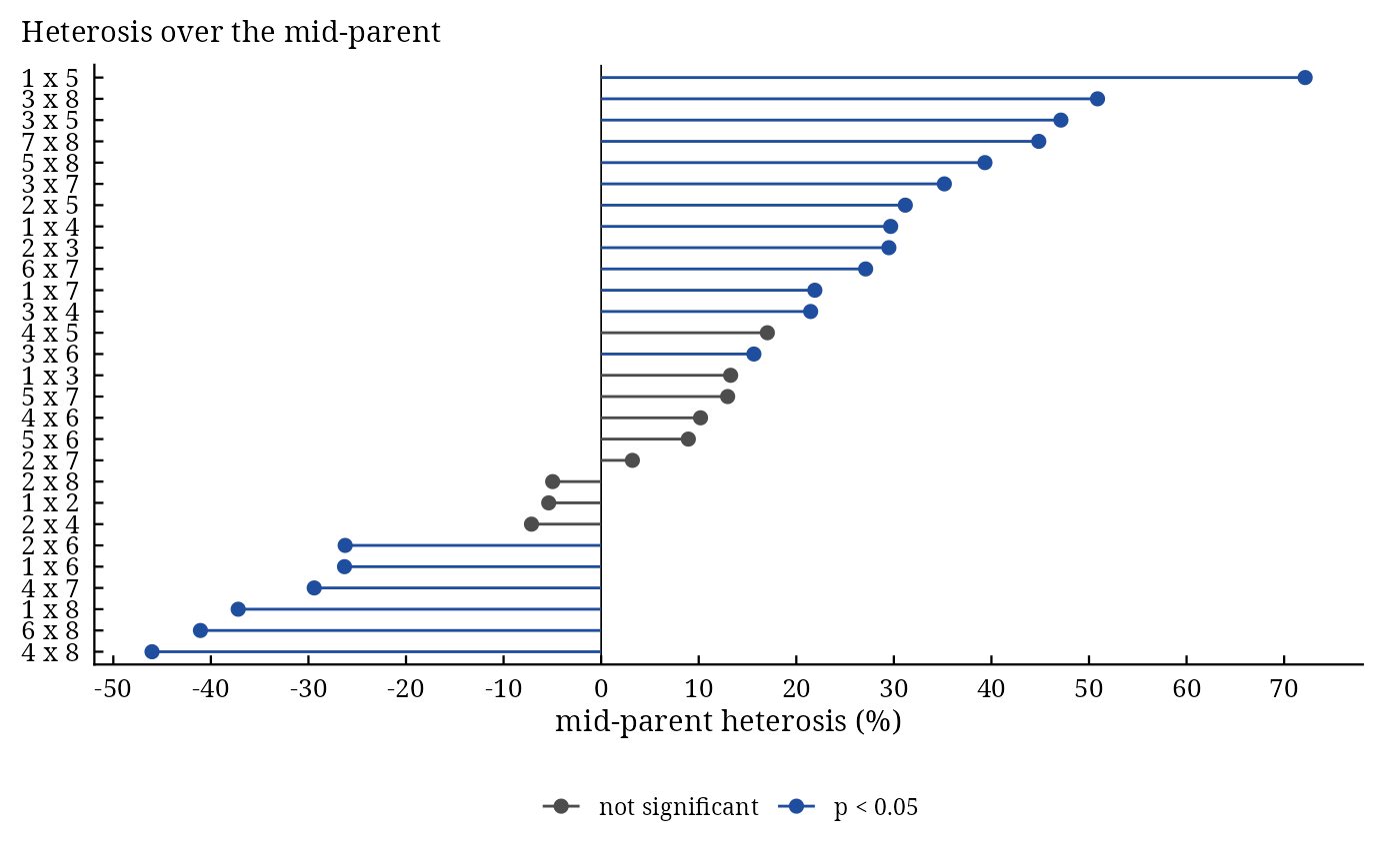
Heterosis over the mid-parent, the better parent and a standard variety
Source:R/Heterosis.R
Heterosis.RdHeterosis() estimates, for every cross of a diallel or a set of crosses grown with their parents in a
randomized complete block experiment, the heterosis over the mid-parent, over the better parent and over a standard
(check) variety, in percent, with \(t\) tests of the underlying differences.
Usage
Heterosis(
  y,
  Rep,
  Cross1,
  Cross2,
  data,
  Check = NULL,
  Better = c("higher", "lower")
)
Arguments
- y
response: a column of
datagiven by name (y = Yieldory = "Yield") or a numeric vector of lengthnrow(data).- Rep
replicate (block): a column of
dataor a vector, as fory.- Cross1
female parent of each plot: a column of
dataor a vector, as fory.- Cross2
male parent of each plot: a column of
dataor a vector, as fory.- data
a data frame (or
data.table) with one row per plot.- Check
label of the standard (check) variety: a parent of the diallel or another entry of
datagrown as a self (Cross1 == Cross2);NULL(default) for no standard heterosis.- Better
"higher"(default) or"lower": which parent is the better one.
Value
An object of class c("da_heterosis", "da_result", "list"):
Meansmatrix of cross means (parents on the diagonal).
Heterosisdata.table, one row per cross:Cross1,Cross2,F1,MidParent,BetterParent,MP(percent),t_MP,p_MP,BP,t_BP,p_BPand, with a check,Check,SH,t_SH,p_SH.StdErrstandard errors of the differences \(F_{ij} - MP\) and \(F_{ij} - BP\) (also used for the check).
RCBDanalysis of variance of the plot data.
Methods: print(), summary(), plot() (heterosis of every cross, significant ones marked;
which = c("MP", "BP", "SH", "residuals", "qq")), data.table::as.data.table(x, component =),
da_export.
Details
Means. \(F_{ij}\) is the mean of cross \(i \times j\) (crosses recorded both ways round
are kept apart, so reciprocal crosses have their own heterosis), \(P_i\) the mean of parent \(i\) and
\(C\) the mean of the check; the means are least-squares means of the block analysis when plots are missing.
With \(B\) replicates and error mean square \(MS_E\) on \(f_E\) degrees of freedom
(Singh and Chaudhary 2004):
$$MP = \frac{P_i + P_j}{2}, \quad H_{MP} = 100\,\frac{F_{ij} - MP}{MP}, \quad t = \frac{F_{ij} - MP}{
\sqrt{3MS_E/(2B)}},$$
$$BP = \max(P_i, P_j), \quad H_{BP} = 100\,\frac{F_{ij} - BP}{BP}, \quad t = \frac{F_{ij} - BP}{
\sqrt{2MS_E/B}},$$
and the standard heterosis \(H_{C} = 100(F_{ij} - C)/C\) with \(t = (F_{ij} -
C)/\sqrt{2MS_E/B}\). For a trait where lower values are better (days to flowering,
disease score) set Better = "lower": the better parent is then the lower one. The p-values are two-sided
on \(f_E\) degrees of freedom.
References
Fonseca, S. and Patterson, F. L. (1968). Hybrid vigor in a seven-parent diallel cross in common winter wheat (Triticum aestivum L.). Crop Science, 8(1), 85–88. doi:10.2135/cropsci1968.0011183X000800010025x
Singh, R. K. and Chaudhary, B. D. (2004). Biometrical Methods in Quantitative Genetic Analysis. Kalyani Publishers, New Delhi.
See also
Other DiallelAnalysisR analyses:
GardnerEberhart(),
Griffing(),
GriffingEnv(),
GriffingMeans(),
Hayman(),
LineTester(),
NCDesign(),
PartialDiallel()
Author
Muhammad Yaseen (myaseen208@gmail.com)
Examples
#-------------------------------------------------------------
## Parents and one set of crosses; parent 3 as the check
#-------------------------------------------------------------
het <-
  Heterosis(
      y      = Yield
    , Rep    = Rep
    , Cross1 = Cross1
    , Cross2 = Cross2
    , data   = GriffingData2
    , Check  = 3
    , Better = c("higher", "lower")[1]
    )
het
#> Heterosis of 28 crosses; check 3
#>
#>     Cross1 Cross2     F1 MidParent BetterParent      MP    t_MP      p_MP
#>     <char> <char>  <num>     <num>        <num>   <num>   <num>     <num>
#>  1:      1      2  87.01     91.95        98.26  -5.375 -0.7637 4.468e-01
#>  2:      1      3  90.45     79.86        85.64  13.271  1.6375 1.045e-01
#>  3:      1      4 114.94     88.64        91.64  29.673  4.0643 9.324e-05
#>  4:      1      5 120.29     69.87        85.64  72.153  7.7903 5.025e-12
#>  5:      1      6  68.55     93.02       100.39 -26.304 -3.7807 2.601e-04
#>  6:      1      7 107.64     88.30        90.96  21.902  2.9884 3.492e-03
#>  7:      1      8  52.64     83.82        85.64 -37.201 -4.8183 4.899e-06
#>  8:      2      3 111.58     86.16        98.26  29.490  3.9263 1.545e-04
#>  9:      2      4  88.17     94.95        98.26  -7.141 -1.0476 2.972e-01
#> 10:      2      5  99.93     76.18        98.26  31.174  3.6697 3.836e-04
#> 11:      2      6  73.27     99.32       100.39 -26.237 -4.0268 1.071e-04
#> 12:      2      7  97.64     94.61        98.26   3.203  0.4682 6.406e-01
#> 13:      2      8  85.65     90.13        98.26  -4.971 -0.6922 4.903e-01
#> 14:      3      4 100.65     82.86        91.64  21.471  2.7489 7.041e-03
#> 15:      3      5  94.28     64.09        74.07  47.122  4.6663 9.086e-06
#> 16:      3      6 100.88     87.23       100.39  15.654  2.1100 3.724e-02
#> 17:      3      7 111.54     82.52        90.96  35.175  4.4849 1.870e-05
#> 18:      3      8 117.74     78.03        82.00  50.875  6.1344 1.532e-08
#> 19:      4      5  85.28     72.87        91.64  17.035  1.9182 5.781e-02
#> 20:      4      6 105.80     96.02       100.39  10.186  1.5112 1.337e-01
#> 21:      4      7  64.45     91.30        91.64 -29.409 -4.1489 6.803e-05
#> 22:      4      8  46.85     86.82        91.64 -46.032 -6.1754 1.267e-08
#> 23:      5      6  84.15     77.25       100.39   8.937  1.0668 2.885e-01
#> 24:      5      7  81.93     72.53        90.96  12.965  1.4531 1.492e-01
#> 25:      5      8  94.82     68.05        82.00  39.336  4.1363 7.131e-05
#> 26:      6      7 121.61     95.68       100.39  27.107  4.0075 1.149e-04
#> 27:      6      8  53.74     91.20       100.39 -41.071 -5.7875 7.476e-08
#> 28:      7      8 125.27     86.48        90.96  44.854  5.9938 2.927e-08
#>     Cross1 Cross2     F1 MidParent BetterParent      MP    t_MP      p_MP
#>     <char> <char>  <num>     <num>        <num>   <num>   <num>     <num>
#>           BP     t_BP      p_BP Check      SH    t_SH      p_SH
#>        <num>    <num>     <num> <num>   <num>   <num>     <num>
#>  1: -11.4492 -1.50545 1.352e-01 74.07  17.470  1.7316 8.628e-02
#>  2:   5.6162  0.64366 5.212e-01 74.07  22.121  2.1926 3.054e-02
#>  3:  25.4310  3.11863 2.345e-03 74.07  55.184  5.4698 3.074e-07
#>  4:  40.4519  4.63613 1.026e-05 74.07  62.400  6.1851 1.211e-08
#>  5: -31.7163 -4.26077 4.456e-05 74.07  -7.452 -0.7387 4.618e-01
#>  6:  18.3405  2.23242 2.771e-02 74.07  45.325  4.4926 1.814e-05
#>  7: -38.5370 -4.41666 2.443e-05 74.07 -28.932 -2.8677 4.998e-03
#>  8:  13.5508  1.78179 7.767e-02 74.07  50.635  5.0188 2.132e-06
#>  9: -10.2687 -1.35022 1.798e-01 74.07  19.036  1.8868 6.194e-02
#> 10:   1.6996  0.22348 8.236e-01 74.07  34.913  3.4605 7.806e-04
#> 11: -27.0196 -3.62981 4.401e-04 74.07  -1.087 -0.1077 9.144e-01
#> 12:  -0.6310 -0.08297 9.340e-01 74.07  31.821  3.1541 2.100e-03
#> 13: -12.8333 -1.68745 9.449e-02 74.07  15.634  1.5496 1.242e-01
#> 14:   9.8265  1.20503 2.309e-01 74.07  35.878  3.5562 5.659e-04
#> 15:  27.2918  2.70513 7.968e-03 74.07  27.292  2.7051 7.968e-03
#> 16:   0.4931  0.06624 9.473e-01 74.07  36.202  3.5883 5.073e-04
#> 17:  22.6253  2.75398 6.940e-03 74.07  50.587  5.0142 2.174e-06
#> 18:  43.5793  4.78199 5.684e-06 74.07  58.951  5.8432 5.814e-08
#> 19:  -6.9347 -0.85041 3.970e-01 74.07  15.141  1.5008 1.364e-01
#> 20:   5.3840  0.72329 4.711e-01 74.07  42.831  4.2454 4.725e-05
#> 21: -29.6704 -3.63851 4.271e-04 74.07 -12.988 -1.2873 2.008e-01
#> 22: -48.8706 -5.99304 2.937e-08 74.07 -36.742 -3.6419 4.222e-04
#> 23: -16.1769 -2.17321 3.201e-02 74.07  13.609  1.3489 1.803e-01
#> 24:  -9.9219 -1.20771 2.299e-01 74.07  10.618  1.0525 2.950e-01
#> 25:  15.6341  1.71555 8.919e-02 74.07  28.014  2.7767 6.504e-03
#> 26:  21.1376  2.83962 5.425e-03 74.07  64.183  6.3617 5.306e-09
#> 27: -46.4688 -6.24261 9.266e-09 74.07 -27.447 -2.7205 7.630e-03
#> 28:  37.7199  4.59130 1.227e-05 74.07  69.124  6.8515 5.140e-10
#>           BP     t_BP      p_BP Check      SH    t_SH      p_SH
#>        <num>    <num>     <num> <num>   <num>   <num>     <num>
#>
#> Standard errors of the differences: F1 - MP 6.472, F1 - BP 7.473
head(het$Heterosis)
#>    Cross1 Cross2       F1 MidParent BetterParent         MP      t_MP
#>    <char> <char>    <num>     <num>        <num>      <num>     <num>
#> 1:      1      2  87.0100  91.95250       98.260  -5.375058 -0.763714
#> 2:      1      3  90.4550  79.85750       85.645  13.270513  1.637523
#> 3:      1      4 114.9450  88.64250       91.640  29.672561  4.064257
#> 4:      1      5 120.2900  69.87375       85.645  72.153348  7.790308
#> 5:      1      6  68.5500  93.01750      100.390 -26.304190 -3.780713
#> 6:      1      7 107.6425  88.30250       90.960  21.901985  2.988413
#>            p_MP         BP       t_BP         p_BP Check       SH       t_SH
#>           <num>      <num>      <num>        <num> <num>    <num>      <num>
#> 1: 4.467504e-01 -11.449216 -1.5054531 1.352100e-01 74.07 17.46996  1.7316057
#> 2: 1.045147e-01   5.616206  0.6436649 5.211962e-01 74.07 22.12097  2.1926089
#> 3: 9.323985e-05  25.431034  3.1186298 2.345241e-03 74.07 55.18429  5.4698131
#> 4: 5.025436e-12  40.451865  4.6361266 1.025726e-05 74.07 62.40043  6.1850706
#> 5: 2.600742e-04 -31.716306 -4.2607669 4.456033e-05 74.07 -7.45241 -0.7386757
#> 6: 3.492189e-03  18.340479  2.2324197 2.771035e-02 74.07 45.32537  4.4926067
#>            p_SH
#>           <num>
#> 1: 8.628077e-02
#> 2: 3.054284e-02
#> 3: 3.074332e-07
#> 4: 1.211061e-08
#> 5: 4.617519e-01
#> 6: 1.814482e-05
plot(x = het, which = c("MP", "BP", "SH", "residuals", "qq")[1])