Diallel analysis by Griffing's methods

Griffing() performs the combining-ability analysis of a diallel cross by the four methods and two models of Griffing (1956): the analysis of variance of general combining ability (gca), specific combining ability (sca) and reciprocal effects, the estimates of the effects with their standard errors (fixed model) or the variance components (random model), from the plot data of a randomized complete block experiment.

Usage

Griffing(
  y,
  Rep,
  Cross1,
  Cross2,
  data,
  Method,
  Model,
  Reciprocal = c("combined", "split")
)

Arguments

y: response: a column of data given by name (y = Yield or y = "Yield") or a numeric vector of length nrow(data).
Rep: replicate (block): a column of data or a vector, as for y.
Cross1: female parent of each plot: a column of data or a vector, as for y.
Cross2: male parent of each plot: a column of data or a vector, as for y.
data: a data frame (or data.table) with one row per plot.
Method: 1 (parents, $F_1$ and reciprocals), 2 (parents and one set of $F_1$), 3 ($F_1$ and reciprocals) or 4 (one set of $F_1$). No default.
Model: 1 (fixed effects) or 2 (random effects). No default.
Reciprocal: "combined" (default; one line for the reciprocal effects, as in earlier versions) or "split": in Methods 1 and 3 the reciprocal line is split into maternal and non-maternal parts (Cockerham and Weir 1977); see Details. Ignored in Methods 2 and 4.

Value

An object of class c("da_griffing", "da_result", "list"), with the components of earlier versions followed by new ones:

Means: $P \times P$ matrix of cell means, female parents in rows, male parents in columns (NA for cells that are not part of the method).
ANOVA: combining-ability analysis of variance (class anova): lines gca, sca, reciprocals (Methods 1 and 3) and Error; columns Df, Sum Sq, Mean Sq, F value, Pr(>F).
Genetic.Components: data frame with one column Components: Model 1 rows gca, sca, Reciprocal (Methods 1, 3), gca/sca; Model 2 rows gca, sca, Reciprocal (Methods 1, 3), Error, Additive, Dominant (Dominance in Method 2), gca/sca.
Effects: (Model 1) $P \times P$ matrix: gca effects on the diagonal, sca effects above it, reciprocal effects below it (Methods 1, 3; NA in Methods 2, 4).
StdErr: (Model 1) named vector of standard errors of effects and of their differences: Method 1 gi, sii, sij, rij, gi_gj, sii_sjj, sii_sij, sii_sjk, sij_sik, sij_skl, rij_rkl; Method 2 gi, sii, sij, gi_gj, sii_sjj, sij_sik, sij_skl; Method 3 gi, sij, rij, gi_gj, sij_sik, sij_skl; Method 4 gi, sij, not_defined, gi_gj, sij_sik, sij_skl.
GCA: (new; Model 1) named vector of gca effects $\hat{\mathbf{g}}$.
SCA: (new; Model 1) symmetric matrix of sca effects, selfs included in Methods 1 and 2.
Reciprocal: (new; Model 1, Methods 1 and 3) matrix of reciprocal effects, $\hat{R}_{ij} = -\hat{R}_{ji}$.
Maternal, NonMaternal: (new; Model 1, Methods 1 and 3, Reciprocal = "split") vector of maternal effects $\hat{\mathbf{m}}$ and matrix of non-maternal effects $\hat{n}_{ij}$; the StdErr vector then also has mi, mi_mj and nij, the ANOVA lines maternal and non-maternal in place of reciprocals, and Genetic.Components the rows Maternal and NonMaternal in place of Reciprocal.
RCBD: (new) analysis of variance of the plot data as a randomized complete block design (lines Rep, Crosses, Residuals).

Methods: print(), summary(), plot() (gca effects with standard-error bars and the sca effects as a heat map, residuals of the block analysis against fitted values, normal quantile plot of the residuals, and a biplot of the cross means; which = c("gca", "sca", "biplot", "residuals", "qq")), anova(), coef(), vcov(), confint(), fitted(), residuals(), predict(), data.table::as.data.table(x, component =); see diallel-methods and da-methods.

Details

Data and cell means. Each plot belongs to a cross $i \times j$ of parents $i$ (female, Cross1) and $j$ (male, Cross2) and to a replicate (block). With $P$ parents and $B$ replicates, the cell means form the $P \times P$ matrix $\mathbf{Y}$ with elements $Y_{ij}$; $Y_{i\cdot}$, $Y_{\cdot j}$ and $Y_{\cdot\cdot}$ are its row, column and grand totals. The four methods differ in the cells present:

Method 1	parents, $F_1$ and reciprocal $F_1$: all $P^2$ cells
Method 2	parents and one set of $F_1$: $P(P+1)/2$ cells
Method 3	$F_1$ and reciprocals, no parents: $P(P-1)$ cells
Method 4	one set of $F_1$ only: $P(P-1)/2$ cells

In Methods 2 and 4 a cross may be recorded either way round (Cross1 = 3, Cross2 = 5 or the reverse); it is stored with the lower-numbered parent first. Every cross of the method must be present; individual plots may be missing. With missing plots the cell means are the least-squares means of the block analysis (block effects summing to zero), which removes the bias a missing plot in a good or a poor block would cause, and $B$ in the error variance of a cell mean is the harmonic mean of the numbers of plots per cross (exact when every cross has the same number of plots, an approximation otherwise).

Model. The mean of cross $i \times j$ is $$Y_{ij} = \mu + g_i + g_j + S_{ij} + R_{ij} + \bar{e}_{ij},$$ with gca effects $\mathbf{g} = (g_1, \ldots, g_P)^\top$, symmetric sca effects $S_{ij} = S_{ji}$ and reciprocal effects $R_{ij} = -R_{ji}$ (Methods 1 and 3 only), and an error of variance $\sigma^2/B$. In the fixed model (Model = 1) the effects are constants with $\sum_i g_i = 0$ and the sca and reciprocal effects summing to zero over each array; in the random model (Model = 2) they are independent random variables with variances $\sigma^2_g$, $\sigma^2_s$ and $\sigma^2_r$.

Error mean square. The plot data are analysed as a randomized complete block design with the crosses as treatments; $MS_E$ is its residual mean square on $f_E$ degrees of freedom. The error line of the combining-ability table is on the scale of a cell mean: sum of squares $SS_E/B$, mean square $\sigma^2_m = MS_E/B$.

Sums of squares (Griffing 1956; Singh and Chaudhary 2004), on the scale of cell means. Method 1: $$SS_g = \frac{1}{2P}\sum_i (Y_{i\cdot} + Y_{\cdot i})^2 - \frac{2}{P^2}Y_{\cdot\cdot}^2, \quad SS_s = \frac{1}{2}\sum_i\sum_j Y_{ij}(Y_{ij} + Y_{ji}) - \frac{1}{2P}\sum_i (Y_{i\cdot} + Y_{\cdot i})^2 + \frac{1}{P^2}Y_{\cdot\cdot}^2, \quad SS_r = \frac{1}{2}\sum_{i<j} (Y_{ij} - Y_{ji})^2,$$ on $P-1$, $P(P-1)/2$ and $P(P-1)/2$ degrees of freedom. Method 2 (totals over the symmetric table, each cross counted once in each of its two arrays): $$SS_g = \frac{1}{P+2}\left[\sum_i (Y_{i\cdot} + Y_{ii})^2 - \frac{4}{P}Y_{\cdot\cdot}^2\right], \quad SS_s = \sum_{i \le j} Y_{ij}^2 - \frac{1}{P+2}\sum_i (Y_{i\cdot} + Y_{ii})^2 + \frac{2}{(P+1)(P+2)}Y_{\cdot\cdot}^2,$$ on $P-1$ and $P(P-1)/2$ degrees of freedom. Method 3: $SS_g = \sum_i (Y_{i\cdot} + Y_{\cdot i})^2/(2(P-2)) - 2Y_{\cdot\cdot}^2/(P(P-2))$, $SS_s = \frac{1}{2}\sum_{i<j}(Y_{ij}+Y_{ji})^2 - \sum_i (Y_{i\cdot} + Y_{\cdot i})^2/(2(P-2)) + Y_{\cdot\cdot}^2/((P-1)(P-2))$ on $P(P-3)/2$ degrees of freedom, $SS_r$ as in Method 1. Method 4: $SS_g = \sum_i Y_{i\cdot}^2/(P-2) - 4Y_{\cdot\cdot}^2/(P(P-2))$, $SS_s = \sum_{i<j} Y_{ij}^2 - \sum_i Y_{i\cdot}^2/(P-2) + 2Y_{\cdot\cdot}^2/((P-1)(P-2))$. These are the sums of squares of the orthogonal least-squares decomposition of the cell means into the gca, sca and reciprocal subspaces, which is how they are computed (one computation for the four methods; the closed forms above are the result).

Tests. Fixed model: every line against $\sigma^2_m$. Random model: gca against sca, sca and reciprocals against $\sigma^2_m$.

Effects (fixed model). Method 1: $\hat{g}_i = (Y_{i\cdot} + Y_{\cdot i})/(2P) - Y_{\cdot\cdot}/P^2$, $\hat{S}_{ij} = (Y_{ij} + Y_{ji})/2 - (Y_{i\cdot} + Y_{\cdot i} + Y_{j\cdot} + Y_{\cdot j})/(2P) + Y_{\cdot\cdot}/P^2$, $\hat{R}_{ij} = (Y_{ij} - Y_{ji})/2$; Methods 2 to 4 analogously (Griffing 1956). The standard errors of the effects and of their differences are $\sqrt{\mathrm{Var}}$ of these linear functions of the cell means with $\sigma^2$ replaced by $MS_E$; for Method 1 for example $\mathrm{Var}(\hat{g}_i) = (P-1)\sigma^2_m/(2P^2)$, $\mathrm{Var}(\hat{S}_{ii}) = (P-1)^2\sigma^2_m/P^2$, $\mathrm{Var}(\hat{S}_{ij}) = (P^2 - 2P + 2)\sigma^2_m/(2P^2)$, $\mathrm{Var}(\hat{R}_{ij}) = \sigma^2_m/2$, $\mathrm{Var}(\hat{g}_i - \hat{g}_j) = \sigma^2_m/P$.

Components. Fixed model, as in Griffing (1956): Method 1 gca $(MS_g - \sigma^2_m)/(2P)$, sca $MS_s - \sigma^2_m$, reciprocal $(MS_r - \sigma^2_m)/2$; Method 2 gca $(MS_g - \sigma^2_m)/(P+2)$, sca $MS_s - \sigma^2_m$; Method 3 gca $(MS_g - \sigma^2_m)/(2(P-2))$, sca $(MS_s - \sigma^2_m)/2$, reciprocal as Method 1; Method 4 gca $(MS_g - \sigma^2_m)/(P-2)$, sca $MS_s - \sigma^2_m$. Random model: the variance components solve the expected mean squares, for Method 1 $$\mathrm{E}(MS_g) = \sigma^2_m + \frac{2(P-1)}{P}\sigma^2_s + 2P\sigma^2_g, \quad \mathrm{E}(MS_s) = \sigma^2_m + \frac{2(P^2-P+1)}{P^2}\sigma^2_s, \quad \mathrm{E}(MS_r) = \sigma^2_m + 2\sigma^2_r,$$ for Method 2 $\mathrm{E}(MS_g) = \sigma^2_m + \sigma^2_s + (P+2)\sigma^2_g$, $\mathrm{E}(MS_s) = \sigma^2_m + \sigma^2_s$; Method 3 $\mathrm{E}(MS_g) = \sigma^2_m + 2\sigma^2_s + 2(P-2)\sigma^2_g$, $\mathrm{E}(MS_s) = \sigma^2_m + 2\sigma^2_s$; Method 4 $\mathrm{E}(MS_g) = \sigma^2_m + \sigma^2_s + (P-2)\sigma^2_g$, $\mathrm{E}(MS_s) = \sigma^2_m + \sigma^2_s$. The coefficients are computed exactly from the design, so they hold for any number of parents. Additive and dominance variances follow as $\sigma^2_A = 2\sigma^2_g$ and $\sigma^2_D = \sigma^2_s$ (non-inbred parents, no epistasis).

Maternal and non-maternal reciprocal effects. With Reciprocal = "split" the reciprocal effect is written $r_{ij} = m_i - m_j + n_{ij}$ (Cockerham and Weir 1977), where $m_i$ is the maternal effect of parent $i$ ($\sum_i m_i = 0$) and $n_{ij} = -n_{ji}$ the non-maternal (specific) reciprocal effect. With $D_{ij} = (\bar{y}_{ij} - \bar{y}_{ji})/2$ the least-squares estimates are $$\hat{m}_i = \frac{1}{P}\sum_{j \neq i} D_{ij}, \qquad \hat{n}_{ij} = D_{ij} - \hat{m}_i + \hat{m}_j,$$ and the reciprocal sum of squares $\sum_{i \neq j} D_{ij}^2$ splits into maternal, $2P\sum_i \hat{m}_i^2$ on $P - 1$ degrees of freedom, and non-maternal, the rest on $(P - 1)(P - 2)/2$. Their expected mean squares are $\sigma^2/B + 2\sigma^2_n + 2P\sigma^2_m$ and $\sigma^2/B + 2\sigma^2_n$, so in Model 2 the maternal line is tested against the non-maternal line and $\hat{\sigma}^2_m = (MS_{mat} - MS_{nm})/(2P)$. The standard errors are $\sqrt{(P - 1)\sigma^2/(2P^2B)}$ for $\hat{m}_i$, $\sqrt{\sigma^2/(PB)}$ for $\hat{m}_i - \hat{m}_j$ and $\sqrt{(P - 2)\sigma^2/(2PB)}$ for $\hat{n}_{ij}$.

Changes from version 0.6.0. The standard errors of Model 1 now use the error mean square; version 0.6.0 used the replicate mean square. In Method 2 the standard errors of $\hat{S}_{ii}$ and $\hat{S}_{ij}$ were swapped in version 0.6.0. In Model 2 of Methods 1 and 3 the reciprocal line is tested on the error degrees of freedom (version 0.6.0 used those of sca for its p-value). The third standard error of Method 4 (a Method 1 formula that has no meaning in Method 4) is NA. The table of means keeps the parents' labels and has every parent in its rows and columns. The sums of squares, tests, effects and components are unchanged.

References

Griffing, B. (1956). Concept of general and specific combining ability in relation to diallel crossing systems. Australian Journal of Biological Sciences, 9(4), 463–493. doi:10.1071/BI9560463

Cockerham, C. C. and Weir, B. S. (1977). Quadratic analyses of reciprocal crosses. Biometrics, 33(1), 187–203. doi:10.2307/2529312

Singh, R. K. and Chaudhary, B. D. (2004). Biometrical Methods in Quantitative Genetic Analysis. Kalyani Publishers, New Delhi.

Author

Muhammad Yaseen (myaseen208@gmail.com), Kent M. Eskridge (keskridge1@unl.edu)

Examples

#-------------------------------------------------------------
## Method 1 (parents, F1 and reciprocals), Model 1 (fixed effects)
#-------------------------------------------------------------
Griffing1Data1 <-
  Griffing(
      y      = Yield
    , Rep    = Rep
    , Cross1 = Cross1
    , Cross2 = Cross2
    , data   = GriffingData1
    , Method = 1
    , Model  = 1
    )
Griffing1Data1
#> Griffing's Method 1, Model 1 (fixed effects); 8 parents, 4 replicates 
#> 
#> Analysis of variance
#>              Df Sum Sq Mean Sq F value Pr(>F)    
#> gca           7   3805   543.5  18.887 <2e-16 ***
#> sca          28  22061   787.9  27.378 <2e-16 ***
#> reciprocals  28    366    13.1   0.454  0.992    
#> Error       189   5439    28.8                   
#> ---
#> Signif. codes:  0 ‘***’ 0.001 ‘**’ 0.01 ‘*’ 0.05 ‘.’ 0.1 ‘ ’ 1
#> 
#> Components
#>            Components
#> gca          32.17142
#> sca         759.10758
#> Reciprocal   -7.86142
#> gca/sca       0.04238
#> 
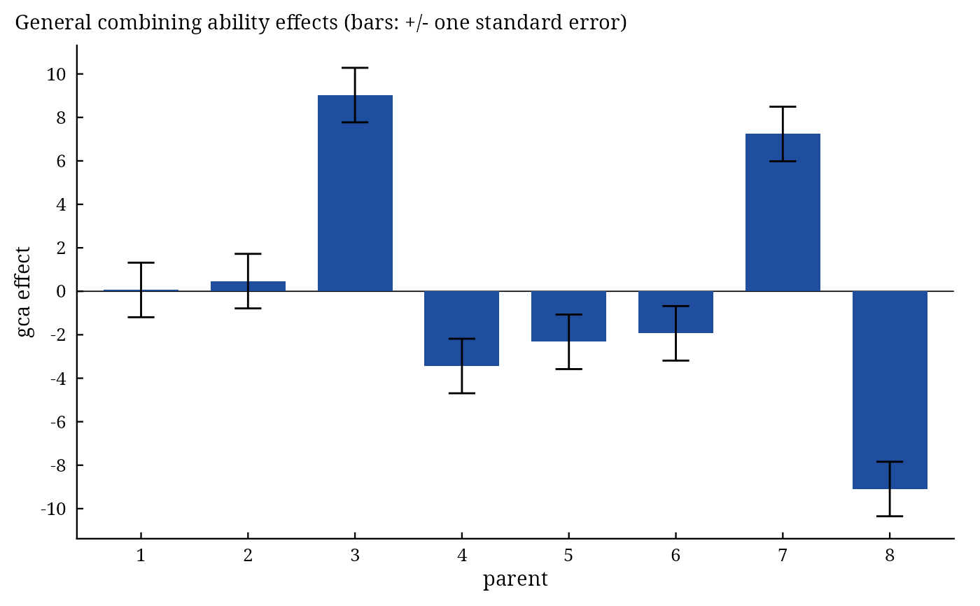
#> General combining ability effects (standard error 1.255)
#>        1        2        3        4        5        6        7        8 
#>  0.06188  0.46800  9.02700 -3.43800 -2.32500 -1.93500  7.23800 -9.09600 
#> 
#> All components: names(x); tests of the effects: summary(x); figures: plot(x)
summary(Griffing1Data1)
#> Griffing's Method 1, Model 1 (fixed effects); 8 parents, 4 replicates 
#> 
#> Analysis of variance
#>              Df Sum Sq Mean Sq F value Pr(>F)    
#> gca           7   3805   543.5  18.887 <2e-16 ***
#> sca          28  22061   787.9  27.378 <2e-16 ***
#> reciprocals  28    366    13.1   0.454  0.992    
#> Error       189   5439    28.8                   
#> ---
#> Signif. codes:  0 ‘***’ 0.001 ‘**’ 0.01 ‘*’ 0.05 ‘.’ 0.1 ‘ ’ 1
#> 
#> Components
#>            Components
#> gca          32.17142
#> sca         759.10758
#> Reciprocal   -7.86142
#> gca/sca       0.04238
#> 
#> General combining ability effects
#>    parent Estimate StdErr  t.value   p.value
#>    <char>    <num>  <num>    <num>     <num>
#> 1:      1  0.06188  1.255  0.04932 9.607e-01
#> 2:      2  0.46797  1.255  0.37303 7.095e-01
#> 3:      3  9.02672  1.255  7.19544 1.420e-11
#> 4:      4 -3.43797  1.255 -2.74050 6.723e-03
#> 5:      5 -2.32547  1.255 -1.85369 6.534e-02
#> 6:      6 -1.93484  1.255 -1.54232 1.247e-01
#> 7:      7  7.23750  1.255  5.76921 3.208e-08
#> 8:      8 -9.09578  1.255 -7.25050 1.034e-11
#> 
#> Crosses with the largest specific combining ability effects
#>    Cross1 Cross2 Estimate StdErr t.value   p.value
#>    <char> <char>    <num>  <num>   <num>     <num>
#> 1:      7      8    32.83  3.353   9.792 1.431e-18
#> 2:      1      4    29.66  3.353   8.846 6.417e-16
#> 3:      1      5    27.30  3.353   8.144 5.072e-14
#> 4:      3      8    25.89  3.353   7.721 6.517e-13
#> 5:      6      7    22.59  3.353   6.737 1.892e-10
Griffing1Data1$ANOVA
#>              Df  Sum Sq Mean Sq F value Pr(>F)    
#> gca           7  3804.6  543.52 18.8868 <2e-16 ***
#> sca          28 22060.8  787.89 27.3783 <2e-16 ***
#> reciprocals  28   365.5   13.05  0.4536 0.9923    
#> Error       189  5439.0   28.78                   
#> ---
#> Signif. codes:  0 ‘***’ 0.001 ‘**’ 0.01 ‘*’ 0.05 ‘.’ 0.1 ‘ ’ 1
Griffing1Data1$StdErr
#>       gi      sii      sij      rij    gi_gj  sii_sjj  sii_sij  sii_sjk 
#> 1.254505 4.693927 3.352805 3.793266 1.896633 6.570129 6.290419 5.689898 
#>  sij_sik  sij_skl  rij_rkl 
#> 5.018019 4.645783 5.364488 
data.table::as.data.table(Griffing1Data1, component = "ANOVA")
#>           term    Df     Sum Sq   Mean Sq    F value       Pr(>F)
#>         <char> <num>      <num>     <num>      <num>        <num>
#> 1:         gca     7  3804.6427 543.52039 18.8868412 5.293328e-19
#> 2:         sca    28 22060.7885 787.88531 27.3783005 3.518704e-52
#> 3: reciprocals    28   365.5369  13.05489  0.4536456 9.923291e-01
#> 4:       Error   189  5438.9907  28.77773         NA           NA
plot(Griffing1Data1)


#-------------------------------------------------------------
## Method 1, Model 2 (random effects)
#-------------------------------------------------------------
Griffing2Data1 <-
  Griffing(
      y      = Yield
    , Rep    = Rep
    , Cross1 = Cross1
    , Cross2 = Cross2
    , data   = GriffingData1
    , Method = 1
    , Model  = 2
    )
Griffing2Data1$Genetic.Components
#>             Components
#> gca        -14.4404522
#> sca        426.1656570
#> Reciprocal  -7.8614195
#> Error       28.7777288
#> Additive   -28.8809045
#> Dominant   426.1656570
#> gca/sca     -0.0338846

#-------------------------------------------------------------
## Method 2 (parents and one set of F1), Model 1
#-------------------------------------------------------------
Griffing1Data2 <-
  Griffing(
      y      = Yield
    , Rep    = Rep
    , Cross1 = Cross1
    , Cross2 = Cross2
    , data   = GriffingData2
    , Method = 2
    , Model  = 1
    )
Griffing1Data2$ANOVA
#>        Df  Sum Sq Mean Sq F value    Pr(>F)    
#> gca     7  1850.9  264.41  9.4698 4.546e-09 ***
#> sca    28 12529.1  447.47 16.0259 < 2.2e-16 ***
#> Error 105  2931.8   27.92                      
#> ---
#> Signif. codes:  0 ‘***’ 0.001 ‘**’ 0.01 ‘*’ 0.05 ‘.’ 0.1 ‘ ’ 1
Griffing1Data2$GCA
#>        1        2        3        4        5        6        7        8 
#> -0.31350  2.38025  5.93025 -2.65325 -4.70575 -0.71825  7.60500 -7.52475 

#-------------------------------------------------------------
## Method 3 (F1 and reciprocals), Model 1
#-------------------------------------------------------------
Griffing1Data3 <-
  Griffing(
      y      = Yield
    , Rep    = Rep
    , Cross1 = Cross1
    , Cross2 = Cross2
    , data   = GriffingData3
    , Method = 3
    , Model  = 1
    )
Griffing1Data3$ANOVA
#>              Df  Sum Sq Mean Sq F value Pr(>F)    
#> gca           7  5612.4  801.78 26.4344 <2e-16 ***
#> sca          20 18336.3  916.82 30.2273 <2e-16 ***
#> reciprocals  28   365.5   13.05  0.4304 0.9948    
#> Error       165  5004.6   30.33                   
#> ---
#> Signif. codes:  0 ‘***’ 0.001 ‘**’ 0.01 ‘*’ 0.05 ‘.’ 0.1 ‘ ’ 1

#-------------------------------------------------------------
## Method 4 (one set of F1), Model 2
#-------------------------------------------------------------
Griffing2Data4 <-
  Griffing(
      y      = Yield
    , Rep    = Rep
    , Cross1 = Cross1
    , Cross2 = Cross2
    , data   = GriffingData4
    , Method = 4
    , Model  = 2
    )
Griffing2Data4$Genetic.Components
#>             Components
#> gca       -3.088483348
#> sca      434.040775861
#> Error     31.187045285
#> Additive  -6.176966696
#> Dominant 434.040775861
#> gca/sca   -0.007115653

Method 1	parents, \(F_1\) and reciprocal \(F_1\): all \(P^2\) cells
Method 2	parents and one set of \(F_1\): \(P(P+1)/2\) cells
Method 3	\(F_1\) and reciprocals, no parents: \(P(P-1)\) cells
Method 4	one set of \(F_1\) only: \(P(P-1)/2\) cells