Bayesian stability analysis: Finlay-Wilkinson, Eberhart-Russell and Shukla models
Source:R/bayes_stability.R
bayes_stability.Rdbayes_stability() fits by Gibbs sampling the joint regression models of Finlay and Wilkinson (1963) and
Eberhart and Russell (1966), and the heterogeneous interaction variance model of Shukla (1972), to the plots of a
multi-environment trial. Every stability parameter (slope, deviation variance, stability variance, safety-first
index) then has a posterior distribution, so genotypes can be compared by probabilities rather than by
significance tests. The data may be unbalanced: plots or whole genotype-environment cells may be missing.
Usage
bayes_stability(
  .data,
  .y,
  .gen,
  .env,
  .rep,
  .model = c("ER", "FW", "Shukla"),
  .nIter = 1000L,
  .burnin = 0L,
  .thin = 1L,
  .chains = 1L,
  .priors = bam_stab_priors(),
  .level = 0.95,
  .alpha = 0.05,
  .seed = NULL,
  .waic = TRUE
)
Arguments
- .data
data frame with one row per plot.
- .y, .gen, .env, .rep
columns of the response, genotype, environment and replicate (bare names or strings).
- .model
"ER"(default),"FW"or"Shukla"; see Details.- .nIter
number of iterations kept per chain before thinning (default 1000).
- .burnin
number of iterations discarded at the start of every chain (default 0).
- .thin
keep every
.thin-th iteration (default 1).- .chains
number of chains (default 1); the first starts at the least-squares estimates, the others at dispersed values.
- .priors
priors from
bam_stab_priors().- .level
probability of the highest posterior density intervals (default 0.95).
- .alpha
probability of the safety-first index (default 0.05, as in Eskridge 1990).
- .seed
seed of the random numbers (the random number state of the session is restored afterwards).
- .waic
compute WAIC during sampling (default
TRUE).
Value
An object of class c("bam_bayes_stability", "bam_result", "list"):
stabilitydata.table, one row per genotype:Gen;mean,mean_lower,mean_upper;slope,slope_lower,slope_upper,prob_slope_above_1;dev_var,dev_var_lower,dev_var_upper;R2;safety_first,safety_first_lower,safety_first_upper,prob_best_safety.environmentsdata.table:Env, posterior mean and HPD interval of the environmental index \(h_j\), and the observed environment mean.summarydata.tableof every parameter (mu,sigma2,g[i],h[j],slope[i],sigma2_d[i]): posterior mean, sd, Monte Carlo error, HPD interval, effective sample size, potential scale reduction factor.drawscoda::mcmc.listof these parameters.deviationsarray (draws x genotypes x environments) of the deviations \(d_{ij}\).
diagnosticsGelman-Rubin, Raftery-Lewis and Heidelberger-Welch diagnostics of the overall mean, error variance, slopes and deviation variances.
fitDIC and WAIC, as in
bayes_ammi().lsleast-squares estimates (the start of the first chain).
settingsiterations, burn-in, thinning, chains, model, priors, level, alpha, seed, time used.
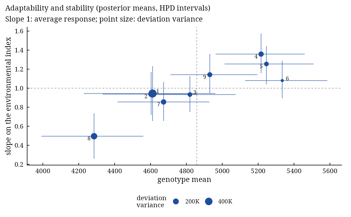
Methods: print(), plot(x, which = c("slopes", "lines", "deviations", "trace", "density")),
bam_interpret(), bam_cite().
Details
For genotype \(i\), environment \(j\) and plot \(l\), $$y_{ijl} = \mu + g_i + (1 + b_i)h_j + d_{ij} + e_{ijl}, \qquad d_{ij} \sim N(0, \sigma^2_{d,i}), \quad e_{ijl} \sim N(0, \sigma^2),$$ with \(\sum_i g_i = \sum_j h_j = \sum_i b_i = 0\). The environment effects \(h_j\) are the environmental index, estimated jointly with the other parameters as in the Bayesian Finlay-Wilkinson regression of Lian and de los Campos (2016) instead of being fixed at the environment means; the slope of genotype \(i\) is \(1 + b_i\), with average 1.
"ER"Eberhart-Russell: slopes and a deviation variance \(\sigma^2_{d,i}\) for every genotype (the Bayesian version of Oliveira et al. 2018). A stable genotype has a slope near 1 and a small deviation variance.
"FW"Finlay-Wilkinson: slopes and one deviation variance for all genotypes.
"Shukla"no slopes (\(b_i = 0\)) and an interaction variance \(\sigma^2_{d,i}\) for every genotype: Shukla's stability variance, as in the Bayesian heterogeneous variance model of Edwards and Jannink (2006).
The sampler draws the overall mean, the genotype effects, the environmental index and the slopes from their
normal conditional distributions with the deviations \(d_{ij}\) integrated out (each observed cell mean
then has variance \(\sigma^2_{d,i} + \sigma^2/n_{ij}\)); then the deviations;
then the variances from their scaled inverse chi-squared conditionals. This partially collapsed Gibbs sampler
mixes well even when the deviations are large. Empty cells contribute no data; their deviations are drawn from the
prior, and bam_predict() predicts them.
stability reports, for every genotype, the posterior mean and HPD interval of its mean
\(\mu + g_i\), slope, deviation variance and the share of its variance across environments explained by
the regression,
\(R^2_i = (1 + b_i)^2 s^2_h / ((1 + b_i)^2 s^2_h + \sigma^2_{d,i})\) with \(s^2_h\) the variance of the environmental index; the posterior probability
that the slope exceeds 1; and the safety-first index of Eskridge (1990),
\(\mu + g_i - z_{1-\alpha}\sqrt{V_i}\), with \(V_i = b_i^2 s^2_h(1 - 1/E) +
\sigma^2_{d,i}\) (Eberhart-Russell), \(b_i^2 s^2_h(1 - 1/E)\) (Finlay-Wilkinson) or \(s^2_h + \sigma^2_{d,i}\) (Shukla). When smaller
values are better (higher_better = FALSE in bam_interpret() and the decision functions), the
index is read the other way: \(\mu + g_i + z_{1-\alpha}\sqrt{V_i}\), smaller better.
The result works with bam_predict(), bam_winners(), bam_superiority(),
bam_ranks(), bam_indices(), bam_compare() and
bam_ppc(), which use the draws of the cell means \(\mu + g_i + (1 + b_i)h_j + d_{ij}\).
References
Finlay, K. W. and Wilkinson, G. N. (1963). The analysis of adaptation in a plant-breeding programme. Australian Journal of Agricultural Research, 14(6), 742–754. doi:10.1071/AR9630742
Eberhart, S. A. and Russell, W. A. (1966). Stability parameters for comparing varieties. Crop Science, 6(1), 36–40. doi:10.2135/cropsci1966.0011183X000600010011x
Shukla, G. K. (1972). Some statistical aspects of partitioning genotype-environmental components of variability. Heredity, 29(2), 237–245. doi:10.1038/hdy.1972.87
Eskridge, K. M. (1990). Selection of stable cultivars using a safety-first rule. Crop Science, 30, 369–374.
Edwards, J. W. and Jannink, J.-L. (2006). Bayesian modeling of heterogeneous error and genotype x environment interaction variances. Crop Science, 46(2), 820. doi:10.2135/cropsci2005.0164
Lian, L. and de los Campos, G. (2016). FW: an R package for Finlay-Wilkinson regression that incorporates genomic/pedigree information and covariance structures between environments. G3: Genes, Genomes, Genetics, 6(3), 589–597. doi:10.1534/g3.115.026328
Oliveira, T. R. A., Carvalho, H. W. L., Nascimento, M., Costa, E. F. N., Amaral Junior, A. T., Gravina, G. A. and Carvalho Filho, J. L. S. (2018). The Eberhart and Russell's Bayesian method used as an instrument to select maize hybrids. Euphytica, 214, 64. doi:10.1007/s10681-018-2146-y
See also
bam_stab_priors, bam_indices, bayes_ammi
Other stability:
bam_ammi_indices(),
bam_indices(),
bam_stab_priors()
Author
Muhammad Yaseen (myaseen208@gmail.com)
Examples
data(Maiz)
fs <-
  bayes_stability(
      .data   = Maiz
    , .y      = y
    , .gen    = entry
    , .env    = site
    , .rep    = rep
    , .model  = "ER"
    , .nIter  = 1000
    , .burnin = 200
    , .thin   = 1
    , .chains = 1
    , .priors = bam_stab_priors(
          mu_var = NULL
        , g_var  = NULL
        , h_var  = NULL
        , b_var  = 100
        , nu     = 1
        , s2     = NULL
        , nu_d   = 1
        , s2_d   = NULL
        )
    , .level  = 0.95
    , .alpha  = 0.05
    , .seed   = 1
    , .waic   = TRUE
    )
fs
#> Bayesian Eberhart-Russell stability model: 9 genotypes, 20 environments, 4 replicates
#> 1 chain(s) x 1000 kept draws (iterations 1000 after a burn-in of 200, thinning 1); 0.3 s
#>
#> Genotypes: posterior means and 95% HPD intervals; safety-first index at alpha = 0.05
#>       Gen  mean mean_lower mean_upper  slope slope_lower slope_upper
#>    <char> <num>      <num>      <num>  <num>       <num>       <num>
#> 1:      1  4612       4228       4961 0.9442      0.6555      1.2310
#> 2:      2  4604       4333       4862 0.9375      0.7197      1.1700
#> 3:      3  4820       4607       5075 0.9331      0.7489      1.1250
#> 4:      4  5216       4963       5459 1.3580      1.1580      1.5750
#> 5:      5  5246       5012       5509 1.2540      1.0400      1.4400
#> 6:      6  5334       5127       5586 1.0800      0.8943      1.2880
#> 7:      7  4673       4416       4928 0.8553      0.6547      1.0660
#> 8:      8  4285       3992       4560 0.4952      0.2577      0.7368
#> 9:      9  4930       4711       5196 1.1420      0.9448      1.3600
#>    prob_slope_above_1 dev_var dev_var_lower dev_var_upper     R2 safety_first
#>                 <num>   <num>         <num>         <num>  <num>        <num>
#> 1:              0.361  494300         34290       1010000 0.7278         3460
#> 2:              0.284  190500         11210        430600 0.8712         3884
#> 3:              0.234  111700         11650        291800 0.9190         4258
#> 4:              0.998  150900         14110        416600 0.9466         4280
#> 5:              0.995  110900         10230        278100 0.9533         4511
#> 6:              0.800   70210         10660        178500 0.9594         4859
#> 7:              0.089  156400          9309        359600 0.8731         3969
#> 8:              0.000  257600         37010        594100 0.5976         3008
#> 9:              0.916  131500         13510        346400 0.9347         4280
#>    safety_first_lower safety_first_upper prob_best_safety
#>                 <num>              <num>            <num>
#> 1:               2757               4228            0.000
#> 2:               3358               4412            0.000
#> 3:               3782               4648            0.003
#> 4:               3812               4739            0.013
#> 5:               4054               4919            0.108
#> 6:               4499               5225            0.856
#> 7:               3498               4447            0.001
#> 8:               2485               3583            0.000
#> 9:               3738               4691            0.019
#>
#> Overall mean 4858, error variance 760500; largest potential scale reduction factor (one chain)
#> All parameters: x$summary; environmental index: x$environments
#>
#> Sources: Eberhart and Russell (1966); Oliveira et al. (2018); Lian and de los
#> Campos (2016); Eskridge (1990); Spiegelhalter et al. (2002); Watanabe (2010).
#> Full references: bam_cite(x).
plot(x = fs, which = "slopes")
#> `height` was translated to `width`.