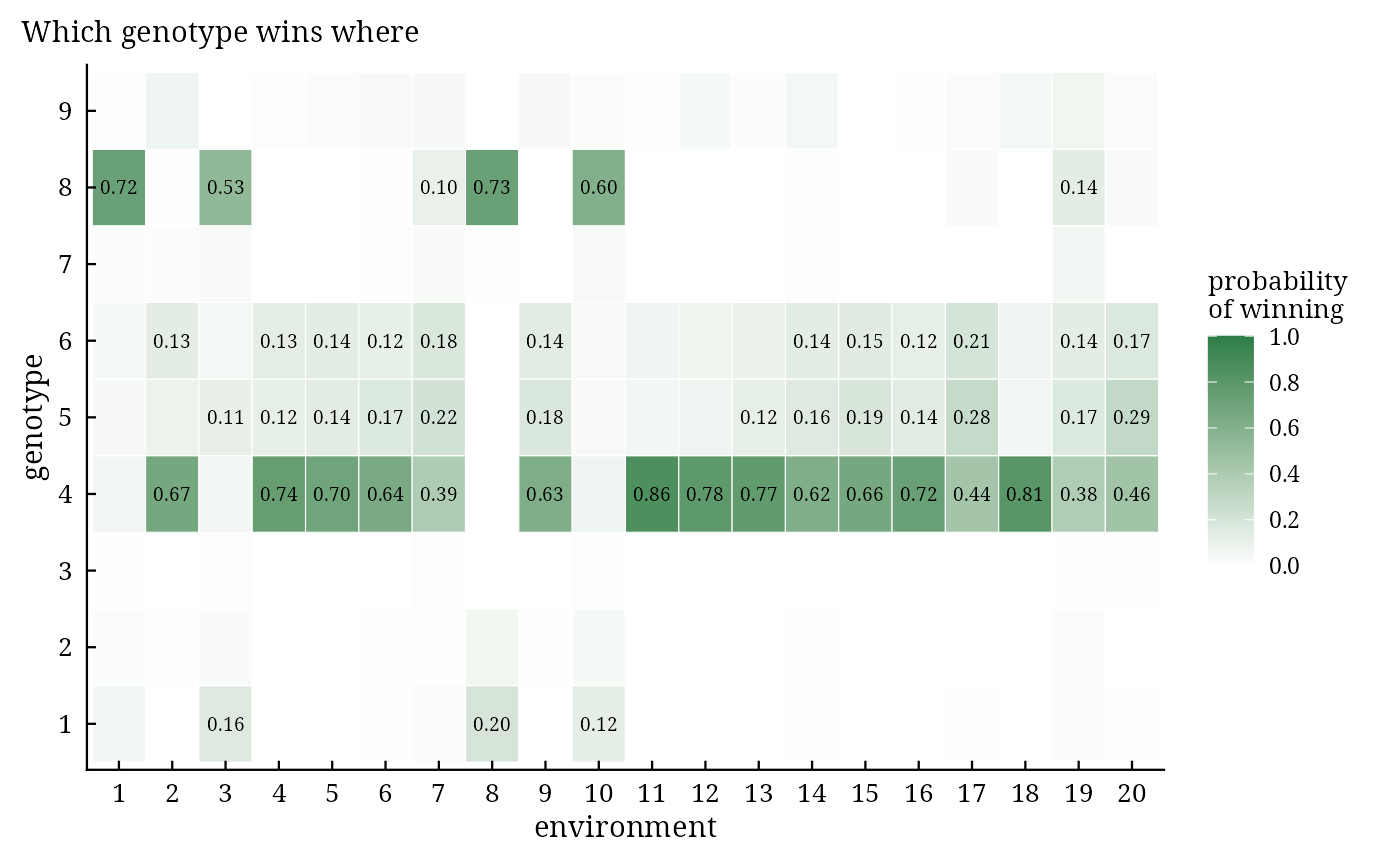
Which genotype wins where: posterior probabilities

bam_winners() gives, for every environment, the posterior probability that each genotype has the best expected response, the most probable winner, and the groups of environments with the same most probable winner (candidate mega-environments). This is the Bayesian counterpart of the which-won-where view of the GGE biplot, with a probability attached to every statement.

Usage

bam_winners(fit, higher_better = TRUE)

Arguments

fit: a result of bayes_ammi() or bayes_stability() (bam_stability() needs bayes_ammi()).
higher_better: TRUE (default) when larger values of the trait are better.

Value

An object of class c("bam_winners", "bam_result", "list"):

probabilities: matrix $G \times E$ of the probabilities $P_{ij}$.
winners: data.table: Env, Winner (most probable), Probability, Second and Probability2 (the runner-up).
mega: data.table: groups of environments with the same most probable winner.

Methods: print(), plot(), bam_interpret().

Details

$$P_{ij} = \Pr\left(\eta_{ij} = \max_{i'}\eta_{i'j} \mid \mathbf{y}\right) \approx \frac{1}{S}\sum_{s=1}^{S} I\left(\eta^{(s)}_{ij} = \max_{i'}\eta^{(s)}_{i'j}\right),$$ with the minimum instead of the maximum when higher_better = FALSE.

References

Yan, W., Hunt, L. A., Sheng, Q. and Szlavnics, Z. (2000). Cultivar evaluation and mega-environment investigation based on the GGE biplot. Crop Science, 40(3), 597–605. doi:10.2135/cropsci2000.403597x

Perez-Elizalde, S., Jarquin, D. and Crossa, J. (2012). A general Bayesian estimation method of linear-bilinear models applied to plant breeding trials with genotype x environment interaction. Journal of Agricultural, Biological, and Environmental Statistics, 17, 15–37. doi:10.1007/s13253-011-0063-9

Author

Muhammad Yaseen (myaseen208@gmail.com)

Examples

data(Maiz)
fit <-
  bayes_ammi(
      .data   = Maiz
    , .y      = y
    , .gen    = entry
    , .env    = site
    , .rep    = rep
    , .nIter  = 1000
    , .k      = 2
    , .burnin = 200
    , .thin   = 1
    , .chains = 1
    , .priors = bam_priors(
          mu_mean     = 0
        , mu_var      = 1e+8
        , tau_mean    = 0
        , tau_var     = 1e+8
        , delta_mean  = 0
        , delta_var   = 1e+8
        , lambda_mean = 0
        , lambda_var  = 1e+8
        , nu          = 1
        , s2          = NULL
        )
    , .level  = 0.95
    , .seed   = 1
    , .align  = TRUE
    , .model  = "GGE"
    , .het    = FALSE
    , .waic   = TRUE
    )
w <-
  bam_winners(
      fit           = fit
    , higher_better = TRUE
    )
w$winners
#>        Env Winner Probability Second Probability2
#>     <char> <char>       <num> <char>        <num>
#>  1:      1      8       0.724      4        0.064
#>  2:      2      4       0.665      6        0.132
#>  3:      3      8       0.534      1        0.157
#>  4:      4      4       0.742      6        0.128
#>  5:      5      4       0.696      5        0.140
#>  6:      6      4       0.644      5        0.165
#>  7:      7      4       0.388      5        0.218
#>  8:      8      8       0.728      1        0.197
#>  9:      9      4       0.628      5        0.179
#> 10:     10      8       0.605      1        0.122
#> 11:     11      4       0.859      6        0.074
#> 12:     12      4       0.782      6        0.083
#> 13:     13      4       0.767      5        0.115
#> 14:     14      4       0.616      5        0.158
#> 15:     15      4       0.664      5        0.186
#> 16:     16      4       0.723      5        0.145
#> 17:     17      4       0.441      5        0.277
#> 18:     18      4       0.807      6        0.080
#> 19:     19      4       0.384      5        0.166
#> 20:     20      4       0.456      5        0.287
#>        Env Winner Probability Second Probability2
#>     <char> <char>       <num> <char>        <num>
plot(x = w)