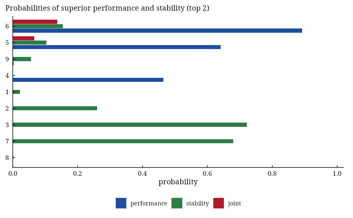
Probabilities of superior performance and stability

bam_superiority() computes the probabilities of Dias et al. (2022) for recommending cultivars: the probability that a genotype is among the best selected fraction across environments and within each environment, the probability that it is among the most stable, their joint probability, and pairwise probabilities that one genotype outperforms or is more stable than another.

Usage

bam_superiority(fit, .s = 0.2, higher_better = TRUE)

Arguments

fit: a result of bayes_ammi() or bayes_stability() (bam_stability() needs bayes_ammi()).
.s: selection intensity: the proportion of genotypes selected (default 0.2).
higher_better: TRUE (default) when larger values of the trait are better.

Value

An object of class c("bam_superiority", "bam_result", "list"):

marginal: data.table sorted by the joint probability: Gen, mean (posterior mean of the marginal value), prob_performance, prob_stability, prob_joint.
conditional: matrix $G \times E$: probability of superior performance in every environment.
pairwise_performance, pairwise_stability: matrices $G \times G$: entry $(i, i')$ is the probability that row genotype $i$ is better (more stable) than $i'$.

Methods: print(), plot() (which = c("marginal", "conditional", "pairwise")), bam_interpret().

Details

With $\Omega^{(s)}$ the $\lceil sG \rceil$ genotypes with the best marginal values $\bar{\eta}^{(s)}_{i\cdot}$ in draw $s$ (selection intensity $s$ = .s), $$P^{\mathrm{perf}}_i = \Pr(i \in \Omega \mid \mathbf{y}), \qquad P^{\mathrm{perf}}_{ij} = \Pr(i \in \Omega_j \mid \mathbf{y}),$$ where $\Omega_j$ selects on $\eta_{ij}$ within environment $j$. Stability is the variance over environments of the interaction effects $ge_{ij} = \eta_{ij} - \bar{\eta}_{i\cdot} - \bar{\eta}_{\cdot j} + \bar{\eta}_{\cdot\cdot}$ (Shukla 1972): $P^{\mathrm{stab}}_i$ is the probability that genotype $i$ is among the $\lceil sG \rceil$ genotypes with the smallest variance, and the joint probability is $P^{\mathrm{perf}}_i P^{\mathrm{stab}}_i$, as in Dias et al. (2022). Pairwise, $\Pr(\bar{\eta}_{i\cdot} > \bar{\eta}_{i'\cdot} \mid \mathbf{y})$ and $\Pr(\mathrm{var}_i < \mathrm{var}_{i'} \mid \mathbf{y})$.

References

Dias, K. O. G., dos Santos, J. P. R., Krause, M. D., Piepho, H.-P., Guimaraes, L. J. M., Pastina, M. M. and Garcia, A. A. F. (2022). Leveraging probability concepts for cultivar recommendation in multi-environment trials. Theoretical and Applied Genetics. doi:10.1007/s00122-022-04041-y

Shukla, G. K. (1972). Some statistical aspects of partitioning genotype-environmental components of variability. Heredity, 29(2), 237–245. doi:10.1038/hdy.1972.87

Author

Muhammad Yaseen (myaseen208@gmail.com)

Examples

data(Maiz)
fit <-
  bayes_ammi(
      .data   = Maiz
    , .y      = y
    , .gen    = entry
    , .env    = site
    , .rep    = rep
    , .nIter  = 1000
    , .k      = 2
    , .burnin = 200
    , .thin   = 1
    , .chains = 1
    , .priors = bam_priors(
          mu_mean     = 0
        , mu_var      = 1e+8
        , tau_mean    = 0
        , tau_var     = 1e+8
        , delta_mean  = 0
        , delta_var   = 1e+8
        , lambda_mean = 0
        , lambda_var  = 1e+8
        , nu          = 1
        , s2          = NULL
        )
    , .level  = 0.95
    , .seed   = 1
    , .align  = TRUE
    , .model  = "AMMI"
    , .het    = FALSE
    , .waic   = TRUE
    )
sp <-
  bam_superiority(
      fit           = fit
    , .s            = 0.2
    , higher_better = TRUE
    )
sp$marginal
#>       Gen     mean prob_performance prob_stability prob_joint
#>    <char>    <num>            <num>          <num>      <num>
#> 1:      6 5331.927            0.892          0.154   0.137368
#> 2:      5 5248.385            0.641          0.104   0.066664
#> 3:      9 4924.780            0.003          0.056   0.000168
#> 4:      4 5219.423            0.464          0.000   0.000000
#> 5:      1 4613.857            0.000          0.022   0.000000
#> 6:      2 4606.430            0.000          0.260   0.000000
#> 7:      3 4822.457            0.000          0.722   0.000000
#> 8:      7 4665.152            0.000          0.680   0.000000
#> 9:      8 4285.844            0.000          0.002   0.000000
plot(x = sp, which = "marginal")