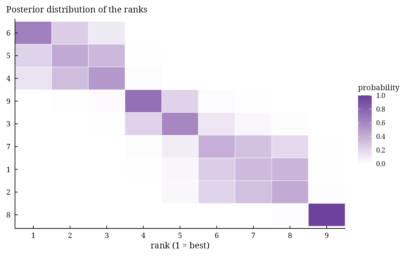
Posterior distribution of the ranks of the genotypes

bam_ranks() gives the posterior probability that each genotype takes each rank, by its mean over the environments (the marginal value) or within one environment, with the expected rank and its HPD interval.

Usage

bam_ranks(fit, higher_better = TRUE, .env = NULL)

Arguments

fit: a result of bayes_ammi() or bayes_stability() (bam_stability() needs bayes_ammi()).
higher_better: TRUE (default) when larger values of the trait are better.
.env: NULL (default: marginal values) or the label of an environment.

Value

An object of class c("bam_ranks", "bam_result", "list"): probabilities (matrix genotypes x ranks) and summary (data.table: Gen, mean_rank, median_rank, lower, upper of the HPD interval of the rank, prob_first). Methods: print(), plot(), bam_interpret().

Details

In draw \(s\) the genotypes are ranked by \(\bar{\eta}^{(s)}_{i\cdot}\) (1 = best); the probability of rank \(r\) is the share of draws in which genotype \(i\) takes it. Ranks summarise the uncertainty of a selection decision better than intervals of the means, since they account for all the genotypes jointly.

References

Dias, K. O. G., dos Santos, J. P. R., Krause, M. D., Piepho, H.-P., Guimaraes, L. J. M., Pastina, M. M. and Garcia, A. A. F. (2022). Leveraging probability concepts for cultivar recommendation in multi-environment trials. Theoretical and Applied Genetics. doi:10.1007/s00122-022-04041-y

Author

Muhammad Yaseen (myaseen208@gmail.com)

Examples

data(Maiz)
fit <-
  bayes_ammi(
      .data   = Maiz
    , .y      = y
    , .gen    = entry
    , .env    = site
    , .rep    = rep
    , .nIter  = 1000
    , .k      = 2
    , .burnin = 200
    , .thin   = 1
    , .chains = 1
    , .priors = bam_priors(
          mu_mean     = 0
        , mu_var      = 1e+8
        , tau_mean    = 0
        , tau_var     = 1e+8
        , delta_mean  = 0
        , delta_var   = 1e+8
        , lambda_mean = 0
        , lambda_var  = 1e+8
        , nu          = 1
        , s2          = NULL
        )
    , .level  = 0.95
    , .seed   = 1
    , .align  = TRUE
    , .model  = "AMMI"
    , .het    = FALSE
    , .waic   = TRUE
    )
rk <-
  bam_ranks(
      fit           = fit
    , higher_better = TRUE
    , .env          = NULL
    )
rk$summary
#>       Gen mean_rank median_rank lower upper prob_first
#>    <char>     <num>       <num> <num> <num>      <num>
#> 1:      6     1.464           1     1     3      0.645
#> 2:      5     2.153           2     1     3      0.215
#> 3:      4     2.417           3     1     3      0.140
#> 4:      9     4.247           4     4     5      0.000
#> 5:      3     4.998           5     3     6      0.000
#> 6:      7     6.553           6     5     8      0.000
#> 7:      1     7.037           7     5     8      0.000
#> 8:      2     7.154           7     5     8      0.000
#> 9:      8     8.977           9     9     9      0.000
plot(x = rk)