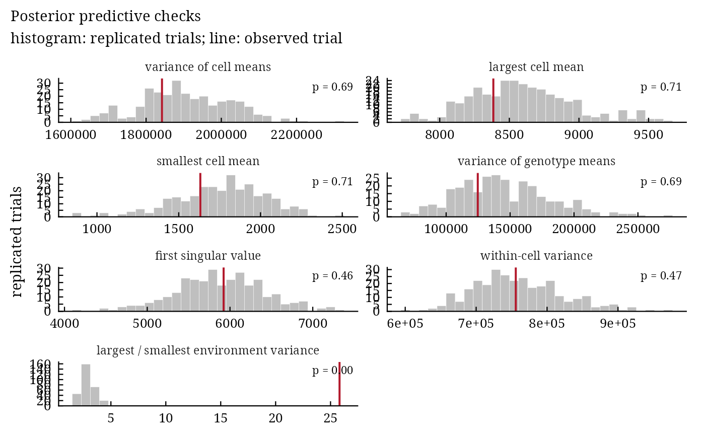
bam_ppc() compares statistics of the observed trial with their distribution in trials replicated from the
posterior predictive distribution (Gelman et al. 1996). A posterior predictive p-value near 0 or 1 shows a feature
of the data that the model does not reproduce, for instance unequal error variances or a missing interaction term.
Arguments
- fit
a result of
bayes_ammi()orbayes_stability().- .draws
number of posterior draws used (default 1000).
- .seed
seed for the replicated trials (the random number state of the session is restored).
Value
An object of class c("bam_ppc", "bam_result", "list") with checks (data.table:
statistic, observed, mean_rep, p_value) and replicated (data.table of
the replicated statistics).
Methods: print(), plot(), bam_interpret().
Details
For a subset of .draws posterior draws, a trial \(\mathbf{y}^{\mathrm{rep}}\) with the observed
plots is simulated from \(N(\eta_{ij}, \sigma^2_j)\), and for each statistic \(T\)
\(p = \Pr(T(\mathbf{y}^{\mathrm{rep}}) \ge T(\mathbf{y}) \mid \mathbf{y})\). The
statistics: variance of the cell means, largest and smallest cell mean, variance of the genotype means, first
singular value of the interaction effects of the cell means, pooled within-cell variance, and the ratio of the
largest to the smallest within-environment variance.
References
Gelman, A., Meng, X.-L. and Stern, H. (1996). Posterior predictive assessment of model fitness via realized discrepancies. Statistica Sinica, 6(4), 733–807.
See also
Other model choice:
bam_compare()
Author
Muhammad Yaseen (myaseen208@gmail.com)
Examples
data(Maiz)
fit <-
  bayes_ammi(
      .data   = Maiz
    , .y      = y
    , .gen    = entry
    , .env    = site
    , .rep    = rep
    , .nIter  = 600
    , .k      = 2
    , .burnin = 100
    , .thin   = 1
    , .chains = 1
    , .priors = bam_priors(
          mu_mean     = 0
        , mu_var      = 1e+8
        , tau_mean    = 0
        , tau_var     = 1e+8
        , delta_mean  = 0
        , delta_var   = 1e+8
        , lambda_mean = 0
        , lambda_var  = 1e+8
        , nu          = 1
        , s2          = NULL
        )
    , .level  = 0.95
    , .seed   = 1
    , .align  = TRUE
    , .model  = "AMMI"
    , .het    = FALSE
    , .waic   = TRUE
    )
pc <-
  bam_ppc(
      fit    = fit
    , .draws = 300
    , .seed  = 1
    )
pc$checks
#>                                  statistic     observed     mean_rep   p_value
#>                                     <char>        <num>        <num>     <num>
#> 1:                  variance of cell means 1.842357e+06 1.904436e+06 0.6866667
#> 2:                       largest cell mean 8.385050e+03 8.597309e+03 0.7066667
#> 3:                      smallest cell mean 1.632000e+03 1.754072e+03 0.7066667
#> 4:              variance of genotype means 1.247327e+05 1.448057e+05 0.6866667
#> 5:                    first singular value 5.922891e+03 5.878150e+03 0.4566667
#> 6:                    within-cell variance 7.558838e+05 7.594279e+05 0.4666667
#> 7: largest / smallest environment variance 2.582038e+01 2.943674e+00 0.0000000
plot(x = pc)