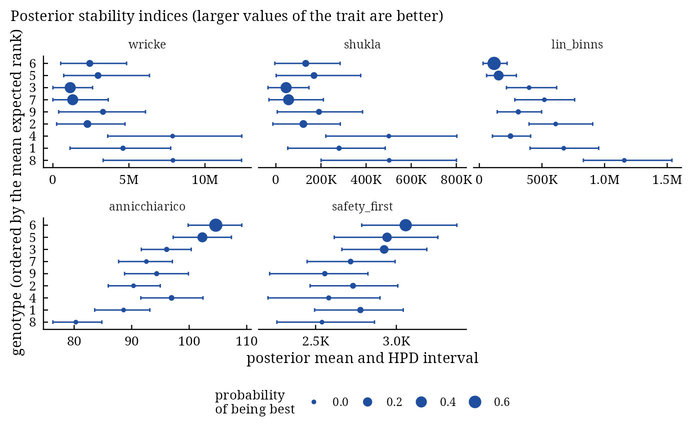
Posterior distributions of classical stability indices

bam_indices() computes five classical stability and superiority indices on every posterior draw of the cell means of a fit, so that each index has a posterior mean, an HPD interval and, for every genotype, a probability of being the best. The indices are those of Wricke (1962), Shukla (1972), Lin and Binns (1988), Annicchiarico (1992) and Eskridge (1990).

Usage

bam_indices(fit, higher_better = TRUE, .prob = 0.25, .alpha = 0.05)

Arguments

fit: a result of bayes_ammi() or bayes_stability().
higher_better: TRUE (default) when larger values of the trait are better.
.prob: error probability \(p\) of Annicchiarico's index (default 0.25).
.alpha: probability \(\alpha\) of the safety-first index (default 0.05).

Value

An object of class c("bam_indices", "bam_result", "list") with

indices: data.table in long form: index, Gen, mean, lower, upper (HPD interval), prob_best (posterior probability that the genotype is the best on this index) and rank_mean (expected rank, 1 = best).
means: data.table: one row per genotype with the posterior means of the indices and the mean of their expected ranks (rank_overall), sorted by it.

Methods: print(), plot(), bam_interpret(), bam_cite().

Details

With \(\eta_{ij}\) the cell mean of genotype \(i\) in environment \(j\) (one posterior draw), \(\bar{\eta}_{i\cdot}\), \(\bar{\eta}_{\cdot j}\) and \(\bar{\eta}_{\cdot\cdot}\) the genotype, environment and overall means, and the interaction \(\epsilon_{ij} = \eta_{ij} - \bar{\eta}_{i\cdot} - \bar{\eta}_{\cdot j} + \bar{\eta}_{\cdot\cdot}\):

wricke: ecovalence \(W_i = \sum_j \epsilon_{ij}^2\); smaller is more stable.
shukla: stability variance \(\sigma^2_i = \frac{G}{(G-2)(E-1)}W_i - \frac{\sum_k W_k}{(G-1)(G-2)(E-1)}\); smaller is more stable.
lin_binns: superiority \(P_i = \sum_j(\eta_{ij} - M_j)^2/(2E)\), \(M_j\) the best cell mean of environment \(j\); smaller is better.
annicchiarico: reliability \(I_i = \bar{Z}_i - z_{1-p}s_{Z_i}\) with \(Z_{ij} = 100\,\eta_{ij}/\bar{\eta}_{\cdot j}\); larger is better (with higher_better = FALSE: \(\bar{Z}_i + z_{1-p}s_{Z_i}\), smaller better).
safety_first: Eskridge's index with the variance across environments, \(\bar{\eta}_{i\cdot} - z_{1-\alpha}s_i\); larger is better (with higher_better = FALSE: \(\bar{\eta}_{i\cdot} + z_{1-\alpha}s_i\), smaller better). bayes_stability() gives the model-based versions of the regression and Shukla models.

Because the indices are computed from the posterior of the cell means, they measure the stability of the expected performance, free of the plot error; the HPD intervals show how well the trial determines them.

References

Wricke, G. (1962). Uber eine Methode zur Erfassung der okologischen Streubreite in Feldversuchen. Zeitschrift fur Pflanzenzuchtung, 47, 92–96.

Shukla, G. K. (1972). Some statistical aspects of partitioning genotype-environmental components of variability. Heredity, 29(2), 237–245. doi:10.1038/hdy.1972.87

Lin, C. S. and Binns, M. R. (1988). A superiority measure of cultivar performance for cultivar x location data. Canadian Journal of Plant Science, 68(1), 193–198. doi:10.4141/cjps88-018

Annicchiarico, P. (1992). Cultivar adaptation and recommendation from alfalfa trials in Northern Italy. Journal of Genetics and Breeding, 46, 269–278.

Eskridge, K. M. (1990). Selection of stable cultivars using a safety-first rule. Crop Science, 30, 369–374.

Author

Muhammad Yaseen (myaseen208@gmail.com)

Examples

data(Maiz)
fit <-
  bayes_ammi(
      .data   = Maiz
    , .y      = y
    , .gen    = entry
    , .env    = site
    , .rep    = rep
    , .nIter  = 600
    , .k      = 2
    , .burnin = 100
    , .thin   = 1
    , .chains = 1
    , .priors = bam_priors(
          mu_mean     = 0
        , mu_var      = 1e+8
        , tau_mean    = 0
        , tau_var     = 1e+8
        , delta_mean  = 0
        , delta_var   = 1e+8
        , lambda_mean = 0
        , lambda_var  = 1e+8
        , nu          = 1
        , s2          = NULL
        )
    , .level  = 0.95
    , .seed   = 1
    , .align  = TRUE
    , .model  = "AMMI"
    , .het    = FALSE
    , .waic   = TRUE
    )
ind <-
  bam_indices(
      fit           = fit
    , higher_better = TRUE
    , .prob         = 0.25
    , .alpha        = 0.05
    )
ind$means
#>       Gen  wricke    shukla lin_binns annicchiarico safety_first rank_overall
#>    <char>   <num>     <num>     <num>         <num>        <num>        <num>
#> 1:      6 2425584 132393.67  117785.8     104.62878     3057.895     2.501667
#> 2:      5 2968303 169119.03  154177.8     102.29537     2942.543     3.195333
#> 3:      3 1139377  45357.12  397179.4      96.08279     2924.692     3.209667
#> 4:      7 1301843  56351.06  519413.6      92.55784     2716.789     4.425667
#> 5:      9 3294210 191172.87  311185.9      94.34320     2556.977     5.294667
#> 6:      2 2271464 121964.49  609427.2      90.31891     2731.834     5.358333
#> 7:      4 7870881 500872.41  248934.1      96.93256     2581.329     6.118000
#> 8:      1 4609697 280190.82  673878.0      88.59706     2777.496     6.480333
#> 9:      8 7893824 502424.96 1157554.5      80.29728     2539.471     8.416333
plot(x = ind)
#> `height` was translated to `width`.