Descriptive Statistics with agricolae
Felipe de Mendiburu1, Muhammad Yaseen2
2020-05-02
Source:vignettes/DescriptiveStats.Rmd
DescriptiveStats.Rmd
- Professor of the Academic Department of Statistics and Informatics of the Faculty of Economics and Planning.National University Agraria La Molina-PERU.
- Department of Mathematics and Statistics, University of Agriculture Faisalabad, Pakistan.
Descriptive statistics
The package agricolae provides some complementary functions to the R program, specifically for the management of the histogram and function hist.
Histogram
The histogram is constructed with the function graph.freq and is associated to other functions: polygon.freq, table.freq, stat.freq. See Figures: @ref(fig:DescriptStats2), @ref(fig:DescriptStats6) and @ref(fig:DescriptStats7) for more details.
Example. Data generated in R . (students’ weight).
weight<-c( 68, 53, 69.5, 55, 71, 63, 76.5, 65.5, 69, 75, 76, 57, 70.5, 71.5, 56, 81.5,
           69, 59, 67.5, 61, 68, 59.5, 56.5, 73, 61, 72.5, 71.5, 59.5, 74.5, 63)
print(summary(weight))
   Min. 1st Qu.  Median    Mean 3rd Qu.    Max.
53.00 59.88 68.00 66.45 71.50 81.50 oldpar<-par(mfrow=c(1,2),mar=c(4,4,0,1),cex=0.6) h1<- graph.freq(weight,col=colors()[84],frequency=1,las=2, ylim=c(0,12),ylab="Frequency") x<-h1$breaks h2<- plot(h1, frequency =2, axes= FALSE,ylim=c(0,0.4),xlab="weight",ylab="Relative (%)") polygon.freq(h2, col=colors()[84], lwd=2, frequency =2) axis(1,x,cex=0.6,las=2) y<-seq(0,0.4,0.1) axis(2, y,y*100,cex=0.6,las=1)
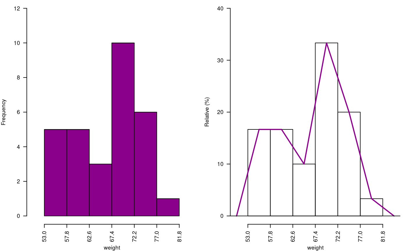
Absolute and relative frequency with polygon
par(oldpar)
Statistics and Frequency tables
Statistics: mean, median, mode and standard deviation of the grouped data.
stat.freq(h1)
$variance
[1] 51.37655

$mean
[1] 66.6

$median
[1] 68.36

$mode
       [-   -]     mode
[1,] 67.4 72.2 70.45455
Frequency tables: Use table.freq, stat.freq and summary
The table.freq is equal to summary()
Limits class: Lower and Upper
Class point: Main
Frequency: Frequency
Percentage frequency: Percentage
Cumulative frequency: CF
Cumulative percentage frequency: CPF
 Lower Upper Main Frequency Percentage CF   CPF
  53.0  57.8 55.4         5       16.7  5  16.7
  57.8  62.6 60.2         5       16.7 10  33.3
  62.6  67.4 65.0         3       10.0 13  43.3
  67.4  72.2 69.8        10       33.3 23  76.7
  72.2  77.0 74.6         6       20.0 29  96.7
  77.0  81.8 79.4         1        3.3 30 100.0
Histogram manipulation functions
You can extract information from a histogram such as class intervals intervals.freq, attract new intervals with the sturges.freq function or to join classes with join.freq function. It is also possible to reproduce the graph with the same creator graph.freq or function plot and overlay normal function with normal.freq be it a histogram in absolute scale, relative or density . The following examples illustrates these properties.
sturges.freq(weight)
$maximum
[1] 81.5

$minimum
[1] 53

$amplitude
[1] 29

$classes
[1] 6

$interval
[1] 4.8

$breaks
[1] 53.0 57.8 62.6 67.4 72.2 77.0 81.8intervals.freq(h1)
     lower upper
[1,]  53.0  57.8
[2,]  57.8  62.6
[3,]  62.6  67.4
[4,]  67.4  72.2
[5,]  72.2  77.0
[6,] 77.0 81.8 Lower Upper Main Frequency Percentage CF CPF
1 53.0 67.4 60.2 13 43.3 13 43.3
2 67.4 72.2 69.8 10 33.3 23 76.7
3 72.2 77.0 74.6 6 20.0 29 96.7
4 77.0 81.8 79.4 1 3.3 30 100.0oldpar<-par(mfrow=c(1,2),mar=c(4,4,0,1),cex=0.8) plot(h3, frequency=2,col=colors()[84],ylim=c(0,0.6),axes=FALSE,xlab="weight",ylab="%") y<-seq(0,0.6,0.2) axis(2,y,y*100,las=2) axis(1,h3$breaks) normal.freq(h3,frequency=2,col=colors()[90]) ogive.freq(h3,col=colors()[84],xlab="weight")
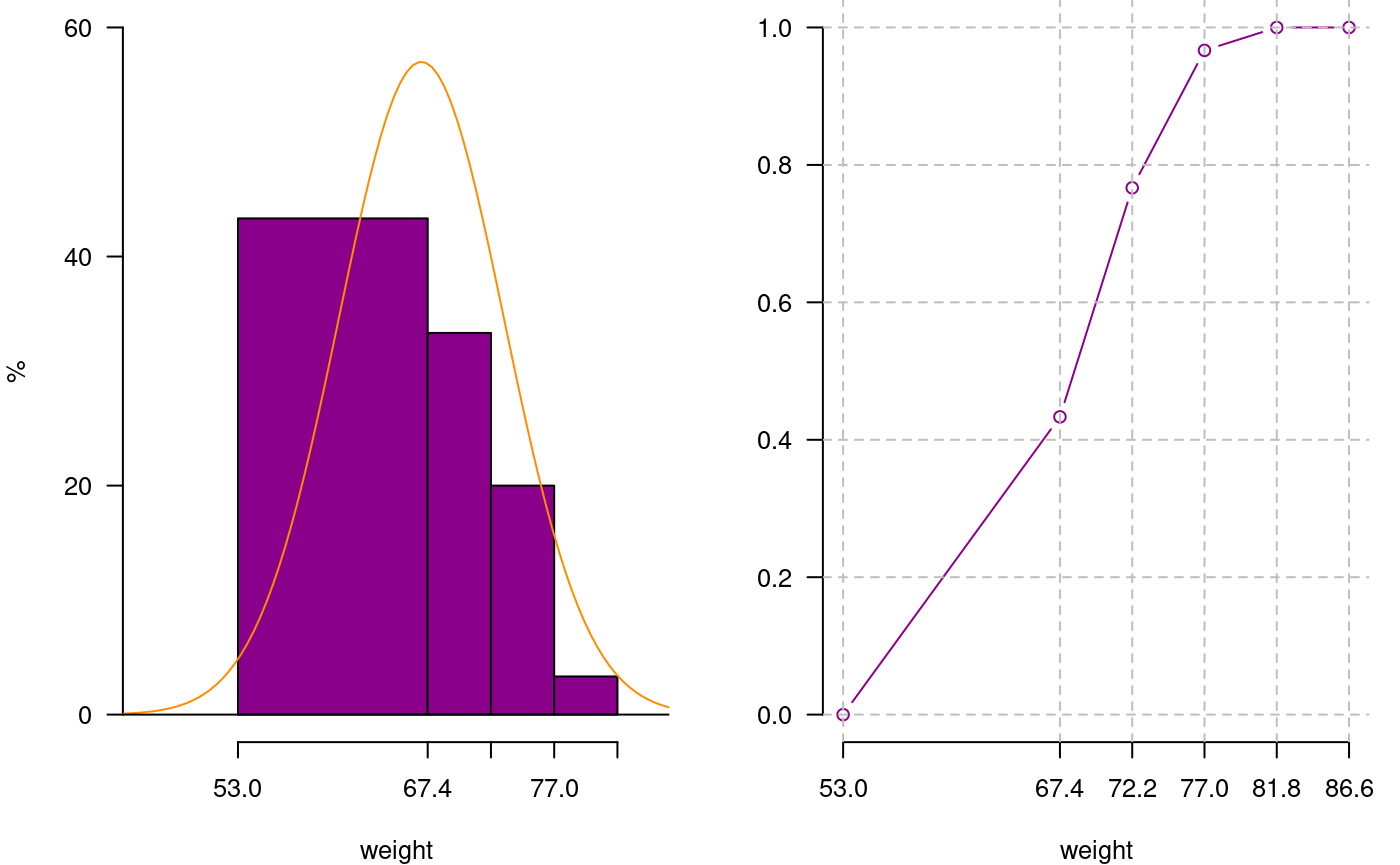
Join frequency and relative frequency with normal and Ogive
  weight    RCF
1   53.0 0.0000
2   67.4 0.4333
3   72.2 0.7667
4   77.0 0.9667
5   81.8 1.0000
6 86.6 1.0000par(oldpar)
hist() and graph.freq() based on grouped data
The hist and graph.freq have the same characteristics, only f2 allows build histogram from grouped data.
0-10 (3)
10-20 (8)
20-30 (15)
30-40 (18)
40-50 (6)
oldpar<-par(mfrow=c(1,2),mar=c(4,3,2,1),cex=0.6)
h4<-hist(weight,xlab="Classes (h4)")
table.freq(h4)
# this is possible
# hh<-graph.freq(h4,plot=FALSE)
# summary(hh)
# new class
classes <- c(0, 10, 20, 30, 40, 50)
freq <- c(3, 8, 15, 18, 6)
h5 <- graph.freq(classes,counts=freq, xlab="Classes (h5)",main="Histogram grouped data")
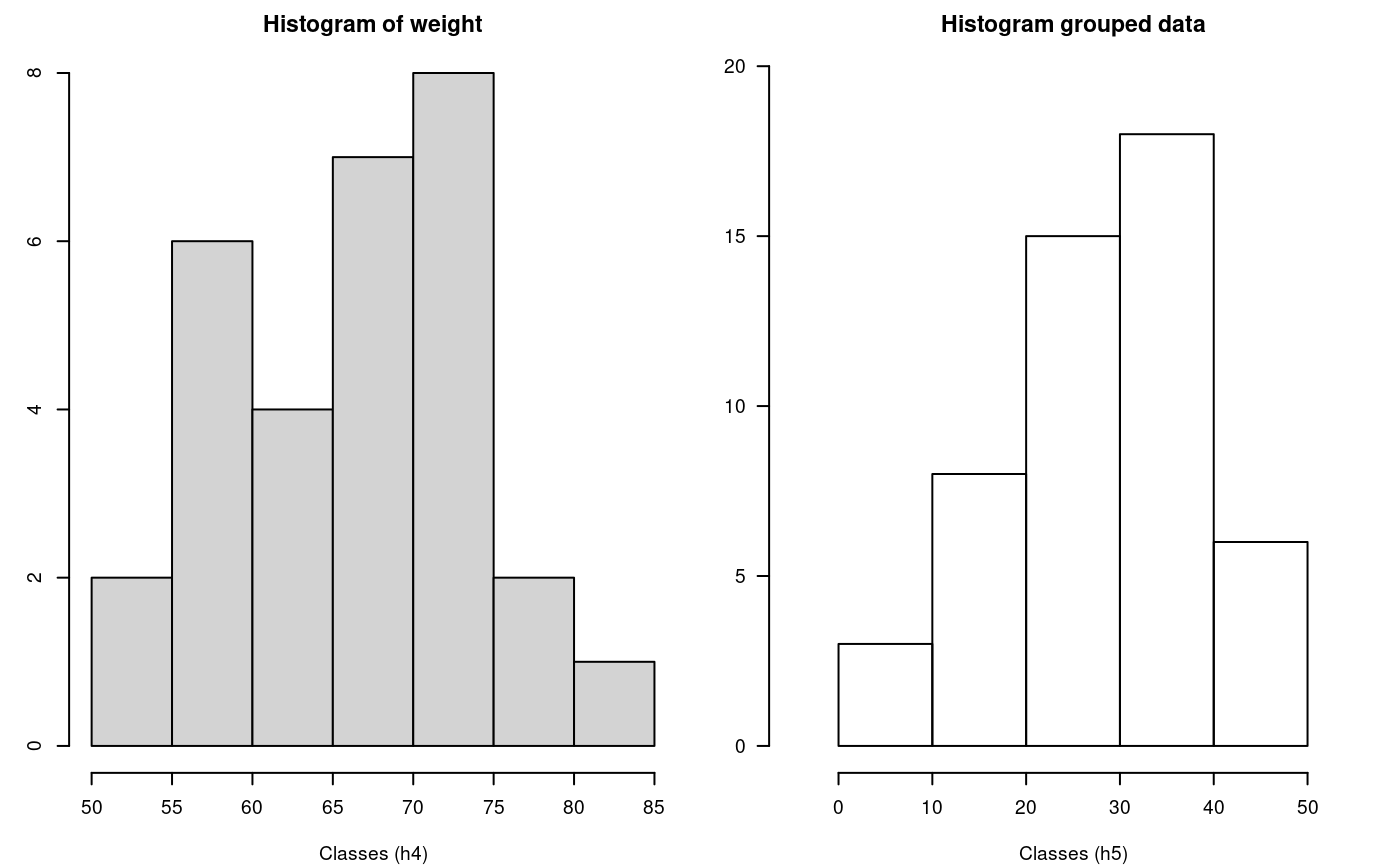
hist() function and histogram defined class
par(oldpar)
 Lower Upper Main Frequency Percentage CF CPF
     0    10    5         3          6  3   6
    10    20   15         8         16 11  22
    20    30   25        15         30 26  52
    30    40   35        18         36 44  88
    40    50   45         6         12 50 100