Introduction to mhpfilter
Muhammad Yaseen
School of Mathematical and Statistical Sciences, Clemson Universitymyaseen208@gmail.com
Javed Iqbal
State Bank of PakistanJaved.iqbal6@sbp.org.pk
M. Nadim Hanif
State Bank of PakistanNadeem.hanif@sbp.org.pk
2026-02-13
Source:vignettes/introduction.Rmd
introduction.RmdOverview
The mhpfilter package provides a fast, efficient
implementation of the Modified Hodrick-Prescott (HP)
filter for decomposing time series into trend and cyclical
components. The key innovation is automatic optimal
selection of the smoothing parameter λ using generalized
cross-validation (GCV), based on the methodology of Choudhary, Hanif
& Iqbal (2014).
Why Modified HP Filter?
The standard HP filter uses fixed λ values:
- λ = 1600 for quarterly data
- λ = 100 for annual data
- λ = 14400 for monthly data
However, these values were calibrated for U.S. quarterly GDP in the 1990s. They may not be appropriate for:
- Different countries (emerging markets vs developed economies)
- Different variables (investment is more volatile than consumption)
- Different time periods (pre/post Great Moderation)
The Modified HP filter solves this by estimating the optimal λ from the data itself using the GCV criterion:
where is the estimated trend for a given , and is the number of observations.
Installation
# Install from GitHub
devtools::install_github("myaseen208/mhpfilter")
Quick Start
Example 1: GDP-like Series
Let’s start with a simulated series that resembles real GDP data:
set.seed(2024)
n <- 120  # 30 years of quarterly data

# Generate components
trend_growth <- 0.005  # 0.5% quarterly growth
trend <- cumsum(c(100, rnorm(n - 1, mean = trend_growth, sd = 0.002)))

# Business cycle: AR(2) process
cycle <- arima.sim(list(ar = c(1.3, -0.5)), n, sd = 2)

# Observed GDP (in logs)
gdp <- trend + cycle

# Apply Modified HP filter
result <- mhp_filter(gdp, max_lambda = 10000)
cat("Optimal lambda:", get_lambda(result), "\n")
#> Optimal lambda: 4337
cat("GCV value:", format(get_gcv(result), digits = 4), "\n")
#> GCV value: 14.36
Visualization with autoplot
result_obj <- mhp_filter(gdp, max_lambda = 10000, as_dt = FALSE)
autoplot(result_obj) +
  labs(
    title = "Modified HP Filter Decomposition of Simulated GDP",
    subtitle = paste0("Optimal λ = ", get_lambda(result_obj))
  ) +
  theme_minimal(base_size = 11) +
  theme(
    plot.title = element_text(face = "bold", size = 13),
    plot.subtitle = element_text(color = "gray40"),
    legend.position = "bottom"
  )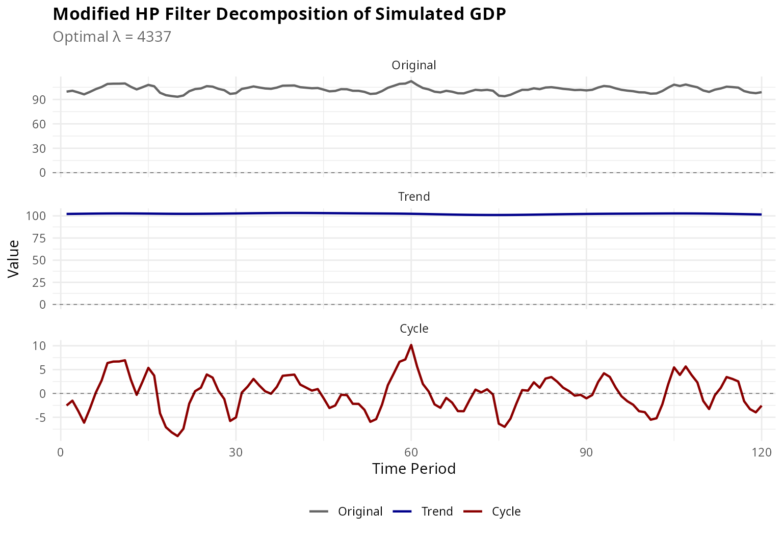
Figure 1: Modified HP Filter Decomposition
Comparison with Standard HP Filter
One of the key features of mhpfilter is the ability to
compare results with the standard HP filter:
Example 2: Why Fixed Lambda Matters
# Apply both filters
mhp_res <- mhp_filter(gdp, max_lambda = 10000)
hp_res <- hp_filter(gdp, lambda = 1600)

# Extract key statistics
comp <- mhp_compare(gdp, frequency = "quarterly", max_lambda = 10000)
print(comp)
#>         method lambda cycle_sd    cycle_mean       ar1 cycle_range      gcv
#>         <char>  <num>    <num>         <num>     <num>       <num>    <num>
#> 1:          HP   1600 3.572060  3.114072e-12 0.7922935    18.43100       NA
#> 2: Modified HP   4337 3.704804 -1.247583e-11 0.8040480    19.11926 14.36441
Visual Comparison
plot_comparison(gdp, frequency = "quarterly", max_lambda = 10000, show_cycle = TRUE) +
  theme_minimal(base_size = 11) +
  theme(
    plot.title = element_text(face = "bold", size = 13),
    legend.position = "bottom",
    legend.box = "vertical"
  )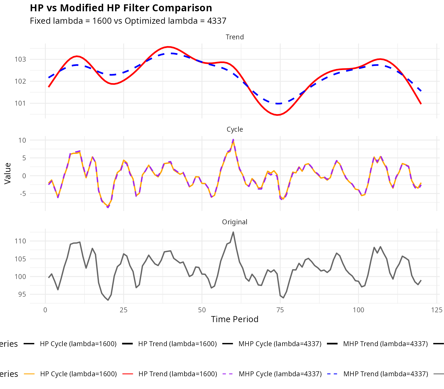
Figure 2: HP vs Modified HP Filter Comparison
Key Insights from Comparison
The comparison reveals important differences:
# Optimal lambda from MHP
opt_lambda <- get_lambda(mhp_res)
cat("Optimal λ (Modified HP):", opt_lambda, "\n")
#> Optimal λ (Modified HP): 4337
cat("Fixed λ (Standard HP):  1600\n\n")
#> Fixed λ (Standard HP):  1600

# Cyclical volatility
sd_mhp <- sd(mhp_res$cycle)
sd_hp <- sd(hp_res$cycle)
cat("Cycle SD (Modified HP):", round(sd_mhp, 3), "\n")
#> Cycle SD (Modified HP): 3.705
cat("Cycle SD (Standard HP):", round(sd_hp, 3), "\n")
#> Cycle SD (Standard HP): 3.572
cat("Difference:", round(sd_mhp - sd_hp, 3),
    paste0("(", round(100 * (sd_mhp - sd_hp) / sd_hp, 1), "%)"), "\n")
#> Difference: 0.133 (3.7%)
Batch Processing: Multi-Country Analysis
A powerful feature is batch processing multiple series simultaneously. This is particularly useful for cross-country macroeconomic comparisons.
Example 3: Cross-Country GDP Comparison
set.seed(456)
n_time <- 100  # 25 years quarterly

# Simulate GDP for multiple countries with different characteristics
countries <- c("USA", "Germany", "Japan", "China", "Brazil", "India")
characteristics <- data.table(
  country = countries,
  trend_growth = c(0.5, 0.4, 0.3, 1.5, 0.6, 1.2),  # % quarterly
  trend_vol = c(0.2, 0.15, 0.15, 0.4, 0.5, 0.6),
  cycle_vol = c(1.5, 1.2, 1.0, 2.5, 3.0, 2.0),
  cycle_ar = c(0.85, 0.88, 0.90, 0.75, 0.70, 0.75)
)

# Generate data
gdp_data <- sapply(1:nrow(characteristics), function(i) {
  char <- characteristics[i, ]
  trend <- 100 + cumsum(rnorm(n_time,
                               mean = char$trend_growth / 100,
                               sd = char$trend_vol / 100))
  cycle <- arima.sim(list(ar = char$cycle_ar), n_time, sd = char$cycle_vol)
  trend + cycle
})
colnames(gdp_data) <- countries

# Apply Modified HP filter to all countries
batch_result <- mhp_batch(gdp_data, max_lambda = 10000)

# View optimal lambdas
lambdas_table <- attr(batch_result, "lambdas")
print(lambdas_table)
#>     series lambda      gcv
#>     <char>  <int>    <num>
#> 1:     USA    566 3.647804
#> 2: Germany    505 3.096862
#> 3:   Japan    389 1.812784
#> 4:   China   1289 7.544833
#> 5:  Brazil   1739 9.723271
#> 6:   India   1464 5.676737
Visualizing Cross-Country Cycles
plot_batch(batch_result, show = "cycle", facet = TRUE) +
  labs(
    title = "Business Cycle Components: Cross-Country Comparison",
    subtitle = "Modified HP Filter with Country-Specific λ",
    caption = "Note: Each country has its own optimal smoothing parameter"
  ) +
  theme_minimal(base_size = 10) +
  theme(
    plot.title = element_text(face = "bold", size = 12),
    strip.text = element_text(face = "bold", size = 9),
    strip.background = element_rect(fill = "gray95", color = "gray80"),
    panel.spacing = unit(0.8, "lines")
  )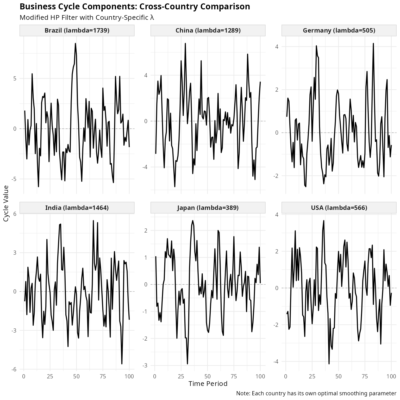
Figure 3: Business Cycles Across Countries
Highlighting Specific Countries
plot_batch(batch_result, show = "cycle", facet = FALSE,
           highlight = c("USA", "China", "India")) +
  labs(
    title = "Business Cycles: Advanced vs Emerging Economies",
    subtitle = "USA (developed) vs China & India (emerging markets)",
    color = "Country (λ)"
  ) +
  theme_minimal(base_size = 11) +
  theme(
    plot.title = element_text(face = "bold", size = 12),
    legend.position = "right",
    legend.key.height = unit(0.8, "lines")
  )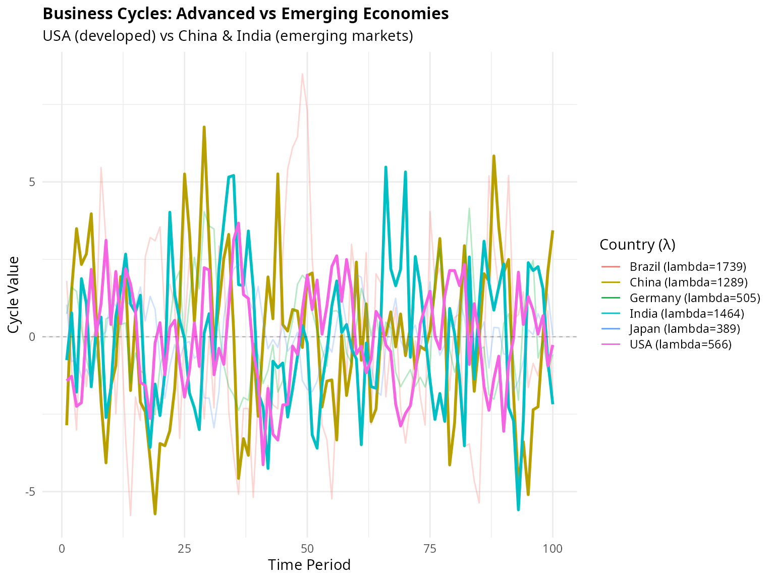
Figure 4: Highlighted Comparison
Batch Comparison with Standard HP
comparison <- batch_compare(gdp_data, frequency = "quarterly", max_lambda = 10000)
print(comparison)
#>     series hp_lambda mhp_lambda hp_cycle_sd mhp_cycle_sd     sd_diff    hp_ar1
#>     <char>     <num>      <int>       <num>        <num>       <num>     <num>
#> 1:     USA      1600        566    1.849002     1.650031 -0.19897143 0.6777133
#> 2: Germany      1600        505    1.728567     1.496906 -0.23166103 0.7346829
#> 3:   Japan      1600        389    1.357226     1.099696 -0.25753039 0.7784002
#> 4:   China      1600       1289    2.606722     2.568540 -0.03818215 0.5954362
#> 5:  Brazil      1600       1739    2.955147     2.967902  0.01275438 0.5726763
#> 6:   India      1600       1464    2.258162     2.246082 -0.01207980 0.5016707
#>      mhp_ar1     ar1_diff relative_sd
#>        <num>        <num>       <num>
#> 1: 0.6111909 -0.066522391   0.8923898
#> 2: 0.6598704 -0.074812412   0.8659809
#> 3: 0.6723097 -0.106090519   0.8102524
#> 4: 0.5828127 -0.012623423   0.9853524
#> 5: 0.5760828  0.003406520   1.0043160
#> 6: 0.4965493 -0.005121396   0.9946506

# Analyze differences
cat("\nSummary of Lambda Differences:\n")
#>
#> Summary of Lambda Differences:
cat("Mean optimal λ:", round(mean(comparison$lambda), 0), "\n")
#> Mean optimal λ: NA
cat("Fixed λ (HP):  1600\n")
#> Fixed λ (HP):  1600
cat("Range of optimal λ:", paste0("[", min(comparison$lambda), ", ",
                                   max(comparison$lambda), "]"), "\n\n")
#> Range of optimal λ: [Inf, -Inf]

cat("Countries with λ > 2000:",
    paste(comparison$series[comparison$lambda > 2000], collapse = ", "), "\n")
#> Countries with λ > 2000:
cat("Countries with λ < 1000:",
    paste(comparison$series[comparison$lambda < 1000], collapse = ", "), "\n")
#> Countries with λ < 1000:
Example 4: Real Business Cycle Analysis
Demonstrating how the Modified HP filter affects business cycle statistics:
# Focus on one country for detailed analysis
usa_gdp <- gdp_data[, "USA"]
usa_mhp <- mhp_filter(usa_gdp, max_lambda = 10000, as_dt = FALSE)
usa_hp <- hp_filter(usa_gdp, lambda = 1600, as_dt = FALSE)

# Create comparison data.table
bc_stats <- data.table(
  Method = c("Modified HP", "Standard HP"),
  Lambda = c(usa_mhp$lambda, 1600),
  `Mean Cycle` = c(mean(usa_mhp$cycle), mean(usa_hp$cycle)),
  `SD Cycle` = c(sd(usa_mhp$cycle), sd(usa_hp$cycle)),
  `Min Cycle` = c(min(usa_mhp$cycle), min(usa_hp$cycle)),
  `Max Cycle` = c(max(usa_mhp$cycle), max(usa_hp$cycle)),
  `AR(1) Coef` = c(
    cor(usa_mhp$cycle[-1], usa_mhp$cycle[-length(usa_mhp$cycle)]),
    cor(usa_hp$cycle[-1], usa_hp$cycle[-length(usa_hp$cycle)])
  )
)

print(bc_stats)
#>         Method Lambda    Mean Cycle SD Cycle Min Cycle Max Cycle AR(1) Coef
#>         <char>  <num>         <num>    <num>     <num>     <num>      <num>
#> 1: Modified HP    566 -6.454571e-13 1.650031 -4.132040  3.671701   0.613421
#> 2: Standard HP   1600  5.820198e-12 1.849002 -4.743509  3.497196   0.683282
Cyclical Properties Visualization
# Create data for plotting
plot_data <- data.table(
  Time = rep(1:n_time, 2),
  Cycle = c(usa_mhp$cycle, usa_hp$cycle),
  Method = rep(c("Modified HP", "Standard HP"), each = n_time),
  Lambda = rep(c(paste0("λ = ", usa_mhp$lambda), "λ = 1600"), each = n_time)
)

ggplot(plot_data, aes(x = Time, y = Cycle, color = Method, linetype = Method)) +
  geom_hline(yintercept = 0, linetype = "dashed", color = "gray60", linewidth = 0.5) +
  geom_line(linewidth = 0.8) +
  scale_color_manual(values = c("Modified HP" = "#0072B2", "Standard HP" = "#D55E00")) +
  scale_linetype_manual(values = c("Modified HP" = "solid", "Standard HP" = "dashed")) +
  labs(
    title = "Business Cycle Components: Method Comparison",
    subtitle = "Modified HP filter allows for data-driven smoothing",
    x = "Time Period (Quarters)",
    y = "Cyclical Component",
    color = NULL,
    linetype = NULL
  ) +
  theme_minimal(base_size = 11) +
  theme(
    plot.title = element_text(face = "bold", size = 12),
    legend.position = "bottom",
    panel.grid.minor = element_blank()
  )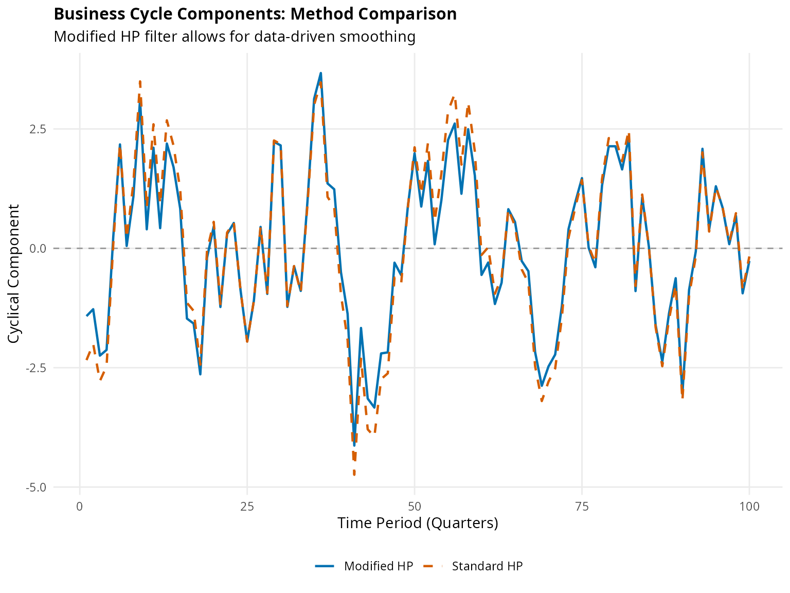
Figure 5: Cyclical Properties Comparison
Example 5: Sensitivity to Lambda
Demonstrating why optimal lambda selection matters:
# Try different lambda values
lambdas_to_try <- c(100, 400, 1600, 6400, get_lambda(mhp_res))
lambda_results <- lapply(lambdas_to_try, function(lam) {
  res <- hp_filter(gdp, lambda = lam, as_dt = FALSE)
  data.table(
    Time = 1:length(gdp),
    Original = gdp,
    Trend = res$trend,
    Cycle = res$cycle,
    Lambda = paste0("λ = ", lam),
    Is_Optimal = lam == get_lambda(mhp_res)
  )
})
sens_data <- rbindlist(lambda_results)

# Plot trends
ggplot(sens_data, aes(x = Time)) +
  geom_line(aes(y = Original), color = "gray60", linewidth = 0.5, alpha = 0.7) +
  geom_line(aes(y = Trend, color = Is_Optimal), linewidth = 0.9) +
  facet_wrap(~Lambda, ncol = 2) +
  scale_color_manual(values = c("TRUE" = "#D55E00", "FALSE" = "#0072B2"),
                     labels = c("Sub-optimal", "Optimal (MHP)"),
                     name = NULL) +
  labs(
    title = "Effect of Lambda on Trend Estimation",
    subtitle = "Lower λ = less smooth (overfitting), Higher λ = too smooth (underfitting)",
    x = "Time Period",
    y = "Value",
    caption = "Gray line shows original series"
  ) +
  theme_minimal(base_size = 10) +
  theme(
    plot.title = element_text(face = "bold", size = 12),
    strip.text = element_text(face = "bold"),
    strip.background = element_rect(fill = "gray95", color = NA),
    legend.position = "bottom",
    panel.spacing = unit(1, "lines")
  )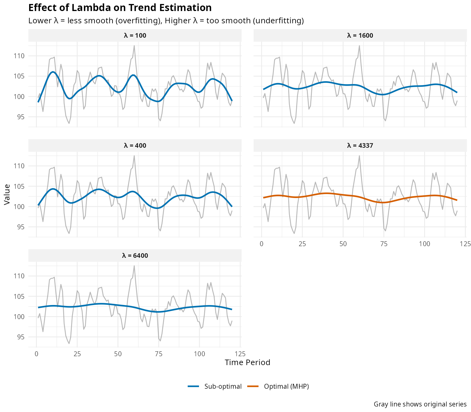
Figure 6: Sensitivity to Lambda Choice
Performance Tips
Choosing max_lambda
The max_lambda parameter determines the search
range:
# For most macroeconomic applications
result_standard <- mhp_filter(gdp, max_lambda = 10000)
cat("Standard search (max_lambda=10000):\n")
#> Standard search (max_lambda=10000):
cat("  Optimal λ:", get_lambda(result_standard), "\n")
#>   Optimal λ: 4337
cat("  GCV:", format(get_gcv(result_standard), digits = 4), "\n\n")
#>   GCV: 14.36

# For very smooth trends or unusual series
result_extended <- mhp_filter(gdp, max_lambda = 50000)
cat("Extended search (max_lambda=50000):\n")
#> Extended search (max_lambda=50000):
cat("  Optimal λ:", get_lambda(result_extended), "\n")
#>   Optimal λ: 4337
cat("  GCV:", format(get_gcv(result_extended), digits = 4), "\n\n")
#>   GCV: 14.36

# Check if we're near the boundary
if (get_lambda(result_standard) > 0.95 * 10000) {
  cat("WARNING: Optimal λ near upper bound. Consider increasing max_lambda.\n")
}
Batch Processing Efficiency
# Efficient for multiple series
large_dataset <- matrix(rnorm(100 * 50), nrow = 100, ncol = 50)
system.time(batch_result <- mhp_batch(large_dataset, max_lambda = 5000))

# Less efficient: loop over columns
system.time({
  manual_result <- lapply(1:50, function(i) {
    mhp_filter(large_dataset[, i], max_lambda = 5000)
  })
})
Summary and Recommendations
When to Use Modified HP Filter
✓ Recommended for:
- Cross-country macroeconomic comparisons
- Analysis of different economic variables (GDP, consumption, investment)
- Uncertain about appropriate λ for your context
- Need defensible, data-driven parameter selection
- Comparing business cycles across countries with different volatility
Standard HP may suffice when:
- Replicating published studies using fixed λ
- U.S. quarterly GDP analysis matching original HP (1997) context
- Speed is critical and λ = 1600 is demonstrably appropriate
Key Takeaways
- Optimal λ varies substantially across countries and variables
- Fixed λ may mis-assign variation to trend vs cycle
- Modified HP filter provides data-driven selection via GCV
- Batch processing enables efficient multi-series analysis
- Visualization tools help understand differences between methods
References
Choudhary, M.A., Hanif, M.N., & Iqbal, J. (2014). On smoothing macroeconomic time series using the modified HP filter. Applied Economics, 46(19), 2205-2214. https://doi.org/10.1080/00036846.2014.896982
Hodrick, R.J., & Prescott, E.C. (1997). Postwar US business cycles: An empirical investigation. Journal of Money, Credit and Banking, 29(1), 1-16.
McDermott, C.J. (1997). An automatic method for choosing the smoothing parameter in the HP filter. Unpublished manuscript, International Monetary Fund.
Ravn, M.O., & Uhlig, H. (2002). On adjusting the Hodrick-Prescott filter for the frequency of observations. Review of Economics and Statistics, 84(2), 371-376.
See Also
-
vignette("methodology", package = "mhpfilter")- Detailed mathematical theory -
?mhp_filter- Main filtering function -
?mhp_batch- Batch processing -
?mhp_compare- Comparison tools