Compare HP vs Modified HP Filter — mhp

Compare the standard HP filter with the Modified HP filter for a single series. Provides summary statistics for both methods including cycle properties.

Usage

mhp_compare(x, frequency = c("quarterly", "annual"), max_lambda = 100000L)

Arguments

x: Numeric vector. The time series to analyze.
frequency: Character. Data frequency: "quarterly" (lambda=1600) or "annual" (lambda=100).
max_lambda: Integer. Maximum lambda for Modified HP search. Default 100000.

Value

A data.table with comparison statistics for both methods:

method: "HP" or "Modified HP"
lambda: Smoothing parameter used
cycle_sd: Standard deviation of cyclical component
cycle_mean: Mean of cyclical component
ar1: First-order autocorrelation of cyclical component
cycle_range: Range of cyclical component (max - min)
gcv: GCV value (NA for standard HP)

Details

The comparison includes: 1. Standard HP filter with fixed lambda (1600 for quarterly, 100 for annual) 2. Modified HP filter with GCV-optimized lambda

Statistics calculated on the cyclical component help assess filter performance: - Lower cycle SD suggests smoother trend - AR(1) near 0 suggests successful cycle extraction - Near-zero mean suggests proper centering

Examples

# Example 1: Quarterly GDP-like series
set.seed(789)
n <- 100
gdp <- cumsum(rnorm(n, mean = 0.7, sd = 0.5)) + 2 * cos(2 * pi * (1:n) / 32)
comparison <- mhp_compare(gdp, frequency = "quarterly", max_lambda = 10000)
print(comparison)
#>         method lambda  cycle_sd    cycle_mean       ar1 cycle_range      gcv
#>         <char>  <num>     <num>         <num>     <num>       <num>    <num>
#> 1:          HP   1600 0.9492746  2.372129e-12 0.8547305    3.882929       NA
#> 2: Modified HP    206 0.5323633 -3.261835e-13 0.6231910    2.408114 0.552981

# Example 2: Annual series
set.seed(101)
n_annual <- 50
annual_series <- cumsum(rnorm(n_annual, mean = 2.0, sd = 1.0)) +
  3 * sin(2 * pi * (1:n_annual) / 10)
annual_comparison <- mhp_compare(annual_series, frequency = "annual", max_lambda = 5000)
print(annual_comparison)
#>         method lambda cycle_sd    cycle_mean       ar1 cycle_range      gcv
#>         <char>  <num>    <num>         <num>     <num>       <num>    <num>
#> 1:          HP    100 2.130999 -2.198952e-13 0.7444730    7.759845       NA
#> 2: Modified HP    956 2.441077  2.926424e-12 0.7834235    9.780873 6.450526

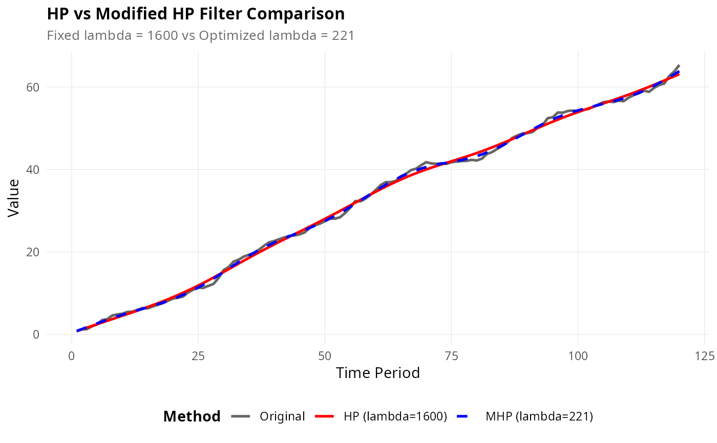
# Example 3: Visual comparison
set.seed(2023)
test_series <- cumsum(rnorm(120, mean = 0.5, sd = 0.4)) +
  runif(1, 1, 3) * sin(2 * pi * (1:120) / 30)

comp_result <- mhp_compare(test_series, frequency = "quarterly", max_lambda = 20000)

if (require(ggplot2)) {
  # Create visualization
  hp_result <- hp_filter(test_series, lambda = 1600, as_dt = FALSE)
  mhp_result <- mhp_filter(test_series, max_lambda = 20000, as_dt = FALSE)

  plot_comparison(test_series, frequency = "quarterly", max_lambda = 20000)
}