Modified HP Filter: Theory and Methodology

Muhammad Yaseen

School of Mathematical and Statistical Sciences, Clemson University
myaseen208@gmail.com

Javed Iqbal

State Bank of Pakistan
Javed.iqbal6@sbp.org.pk

M. Nadim Hanif

State Bank of Pakistan
Nadeem.hanif@sbp.org.pk

2026-02-13

Introduction

This vignette provides a detailed explanation of the methodology underlying the Modified Hodrick-Prescott (HP) filter as implemented in the mhpfilter package. We cover the mathematical foundations, the cross-validation approach for optimal parameter selection, and empirical evidence supporting its use.

library(mhpfilter)
#> mhpfilter 0.1.0 loaded
library(fastverse)
#> -- Attaching packages --------------------------------------- fastverse 0.3.4 --
#> v data.table 1.18.2.1     v kit        0.0.21  
#> v magrittr   2.0.4        v collapse   2.1.6
library(tidyverse)
#> ── Attaching core tidyverse packages ──────────────────────── tidyverse 2.0.0 ──
#> ✔ dplyr     1.2.0     ✔ readr     2.1.6
#> ✔ forcats   1.0.1     ✔ stringr   1.6.0
#> ✔ ggplot2   4.0.2     ✔ tibble    3.3.1
#> ✔ lubridate 1.9.5     ✔ tidyr     1.3.2
#> ✔ purrr     1.2.1
#> ── Conflicts ────────────────────────────────────────── tidyverse_conflicts() ──
#> ✖ dplyr::between()     masks data.table::between()
#> ✖ dplyr::count()       masks kit::count()
#> ✖ tidyr::extract()     masks magrittr::extract()
#> ✖ dplyr::filter()      masks stats::filter()
#> ✖ dplyr::first()       masks data.table::first()
#> ✖ lubridate::hour()    masks data.table::hour()
#> ✖ lubridate::isoweek() masks data.table::isoweek()
#> ✖ lubridate::isoyear() masks data.table::isoyear()
#> ✖ dplyr::lag()         masks stats::lag()
#> ✖ dplyr::last()        masks data.table::last()
#> ✖ lubridate::mday()    masks data.table::mday()
#> ✖ lubridate::minute()  masks data.table::minute()
#> ✖ lubridate::month()   masks data.table::month()
#> ✖ lubridate::quarter() masks data.table::quarter()
#> ✖ tidyr::replace_na()  masks collapse::replace_na()
#> ✖ lubridate::second()  masks data.table::second()
#> ✖ purrr::set_names()   masks magrittr::set_names()
#> ✖ purrr::transpose()   masks data.table::transpose()
#> ✖ lubridate::wday()    masks data.table::wday()
#> ✖ lubridate::week()    masks data.table::week()
#> ✖ lubridate::yday()    masks data.table::yday()
#> ✖ lubridate::year()    masks data.table::year()
#> ℹ Use the conflicted package (<http://conflicted.r-lib.org/>) to force all conflicts to become errors

1. The Standard HP Filter

1.1 Problem Formulation

The Hodrick-Prescott (1997) filter decomposes a time series $y_t$ into a trend component $g_t$ and a cyclical component $c_t$:

$$y_t = g_t + c_t, \quad t = 1, 2, \ldots, T$$

The filter estimates the trend by solving the optimization problem:

$$\min_{g_t} \left\{ \sum_{t=1}^{T}(y_t - g_t)^2 + \lambda \sum_{t=3}^{T}[(g_t - g_{t-1}) - (g_{t-1} - g_{t-2})]^2 \right\}$$

This objective function balances two competing goals:

1. Goodness of fit: $\sum_{t=1}^{T}(y_t - g_t)^2$ - the trend should be close to the data
2. Smoothness: $\sum_{t=3}^{T}(\Delta^2 g_t)^2$ - the trend’s growth rate should not change too rapidly

The smoothing parameter $\lambda$ controls the trade-off:

• $\lambda \to 0$: Trend equals original series (no smoothing)
• $\lambda \to \infty$: Trend is a linear time trend (maximum smoothing)

1.2 Matrix Formulation

The solution can be expressed in matrix form. Define the second-difference operator matrix $K$ of dimension $(T-2) \times T$:

$$K = \begin{pmatrix} 1 & -2 & 1 & 0 & \cdots & 0 \\ 0 & 1 & -2 & 1 & \cdots & 0 \\ \vdots & & \ddots & \ddots & \ddots & \vdots \\ 0 & \cdots & 0 & 1 & -2 & 1 \end{pmatrix}$$

Let $A = K'K$. Then the HP filter solution is:

$$\hat{g} = (I + \lambda A)^{-1} y$$

where $I$ is the $T \times T$ identity matrix.

1.3 The Problem with Fixed Lambda

Hodrick and Prescott (1997) recommended $\lambda = 1600$ for quarterly U.S. GDP data, based on the assumption that:

“A 5 percent cyclical component is moderately large, as is one-eighth of 1 percent change in the growth rate in a quarter.”

This led to $\lambda = (5 / 0.125)^2 = 1600$.

However, this assumption may not hold for:

• Different countries (emerging markets have more volatile cycles)
• Different series (investment is more volatile than consumption)
• Different time periods (Great Moderation vs earlier periods)

set.seed(100)
y <- cumsum(rnorm(80)) + 2*sin((1:80)*pi/20)

lambdas <- c(100, 400, 1600, 6400)

# Create data frame for all lambda values
plot_data <- data.frame()

for (lam in lambdas) {
  result <- hp_filter(y, lambda = lam)
  
  temp_data <- data.frame(
    time = rep(1:length(y), 2),
    value = c(y, result$trend),
    series = rep(c("Original", "Trend"), each = length(y)),
    lambda = paste("λ =", lam)
  )
  
  plot_data <- rbind(plot_data, temp_data)
}

# Create faceted plot with combined legend
ggplot(plot_data, aes(x = time, y = value, color = series, linewidth = series)) +
  geom_line() +
  scale_color_manual(values = c("Original" = "black", "Trend" = "blue")) +
  scale_linewidth_manual(values = c("Original" = 0.7, "Trend" = 1.2)) +
  facet_wrap(~ lambda, ncol = 2) +
  labs(x = "Time", y = "Value", color = "Series", linewidth = "Series") +
  theme_minimal() +
  theme(legend.position = "bottom",
        strip.text = element_text(size = 10, face = "bold"))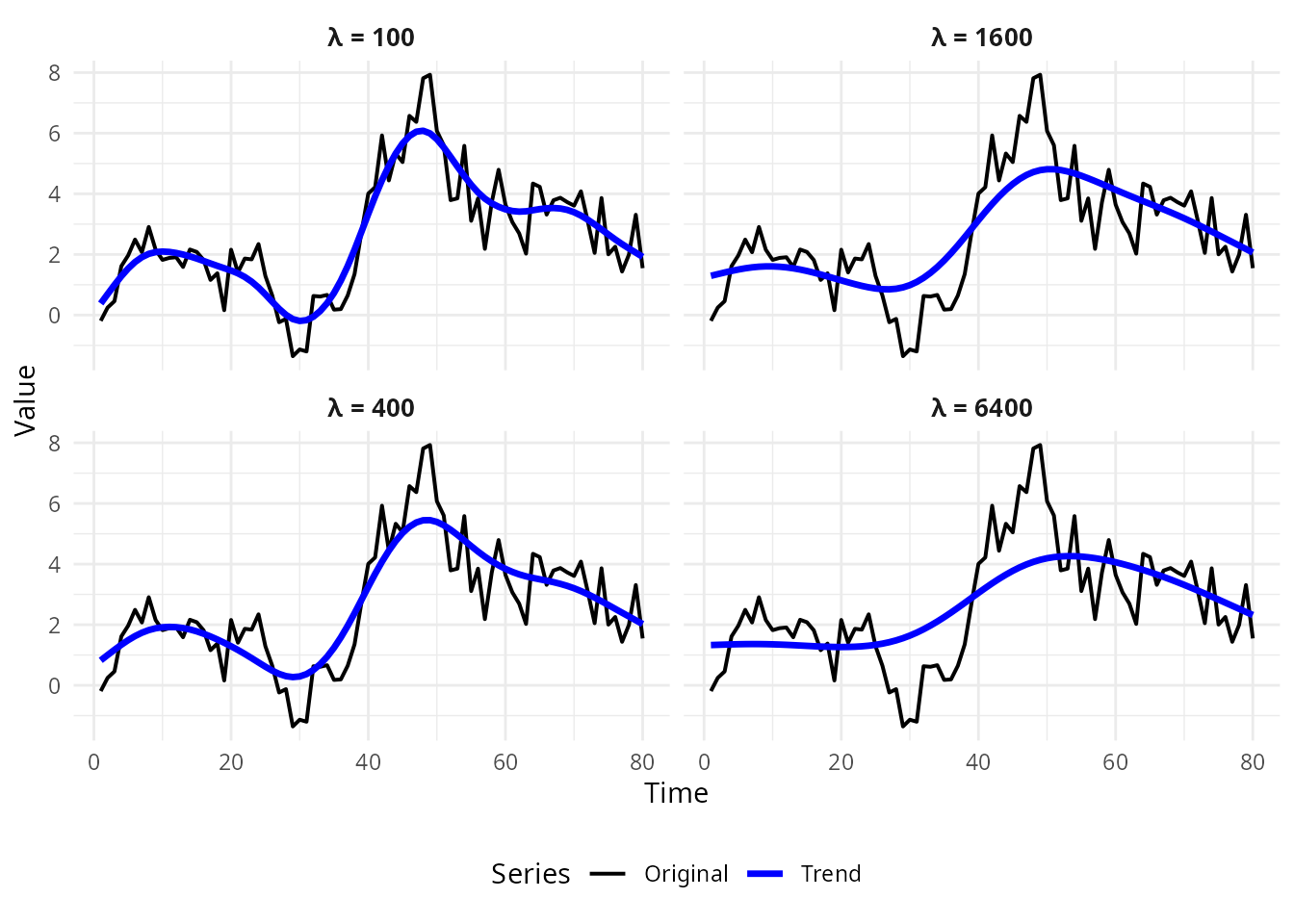

Effect of Lambda on Trend Smoothness

2. The Modified HP Filter

2.1 Cross-Validation Approach

The Modified HP filter, developed by McDermott (1997) and applied empirically by Choudhary, Hanif & Iqbal (2014), selects $\lambda$ using generalized cross-validation (GCV).

The idea is based on leave-one-out cross-validation:

1. For each observation $k$, fit the HP filter to all data except $y_k$
2. Predict the left-out observation using the fitted trend
3. Choose $\lambda$ that minimizes the average prediction error

Let $g_{T,\lambda}^{(k)}(t_k)$ denote the predicted value at time $k$ from the spline fitted leaving out observation $k$. The cross-validation function is:

$$CV(\lambda) = \frac{1}{T} \sum_{k=1}^{T} \left(y_k - g_{T,\lambda}^{(k)}(t_k)\right)^2$$

2.2 Generalized Cross-Validation

Computing the leave-one-out CV is computationally intensive. Craven & Wahba (1979) showed it can be approximated by the generalized cross-validation (GCV) function:

$$GCV(\lambda) = \frac{T^{-1} \sum_{k=1}^{T}(y_k - g_{t,k}^\lambda)^2}{\left(1 - \frac{1}{T}\text{tr}(B(\lambda))\right)^2}$$

where $B(\lambda) = (I + \lambda A)^{-1}$ is the “hat matrix” and $g_{t,k}^\lambda = \sum_{s=1}^{T} b_{ks}(\lambda) y_s$.

Using Silverman’s (1984) approximation for the trace:

$$\text{tr}(B(\lambda)) \approx \frac{T}{\lambda}$$

This yields the simplified GCV formula used in this package:

$$GCV(\lambda) = T^{-1} \left(1 + \frac{2T}{\lambda}\right) \sum_{k=1}^{T}(y_k - g_{t,k}^\lambda)^2$$

2.3 Algorithm

The algorithm implemented in mhpfilter is:

1. Compute $A = K'K$ once (shared across all $\lambda$ values)
2. For $\lambda = 1, 2, \ldots, \lambda_{max}$:
   • Compute trend: $g = (I + \lambda A)^{-1} y$
   • Compute residuals: $r = y - g$
   • Compute GCV: $GCV(\lambda) = T^{-1}(1 + 2T/\lambda) \cdot r'r$
3. Select $\lambda^* = \arg\min_\lambda GCV(\lambda)$
4. Return final decomposition using $\lambda^*$

set.seed(42)
y <- cumsum(rnorm(100, 0.5, 0.3)) + arima.sim(list(ar = 0.8), 100)

# Compute GCV for range of lambdas
lambdas <- seq(100, 5000, by = 50)
gcv_values <- sapply(lambdas, function(lam) {
  res <- hp_filter(y, lambda = lam, as_dt = FALSE)
  T <- length(y)
  resid_ss <- sum((y - res$trend)^2)
  (1 + 2*T/lam) * resid_ss / T
})

# Create data frame for plotting
plot_data <- data.frame(
  lambda = lambdas,
  gcv = gcv_values
)

# Find minimum
opt_idx <- which.min(gcv_values)
opt_lambda <- lambdas[opt_idx]
opt_gcv <- gcv_values[opt_idx]

# Create ggplot
ggplot(plot_data, aes(x = lambda, y = gcv)) +
  geom_line(linewidth = 1.2) +
  geom_vline(xintercept = opt_lambda, color = "red", linetype = "dashed", linewidth = 0.8) +
  geom_point(data = data.frame(lambda = opt_lambda, gcv = opt_gcv), 
             aes(x = lambda, y = gcv), 
             color = "red", size = 3) +
  # Corrected: Use annotate() instead of geom_label() with aes()
  annotate("label",
           x = opt_lambda + 500, 
           y = max(gcv_values) * 0.95,
           label = paste("Optimal λ =", opt_lambda),
           color = "red",
           fill = "white",
           size = 4) +
  labs(
    x = expression(lambda),
    y = "GCV",
    title = "Generalized Cross-Validation Function"
  ) +
  theme_minimal() +
  theme(
    plot.title = element_text(hjust = 0.5, size = 14, face = "bold"),
    axis.title = element_text(size = 12),
    panel.grid.minor = element_blank()
  )

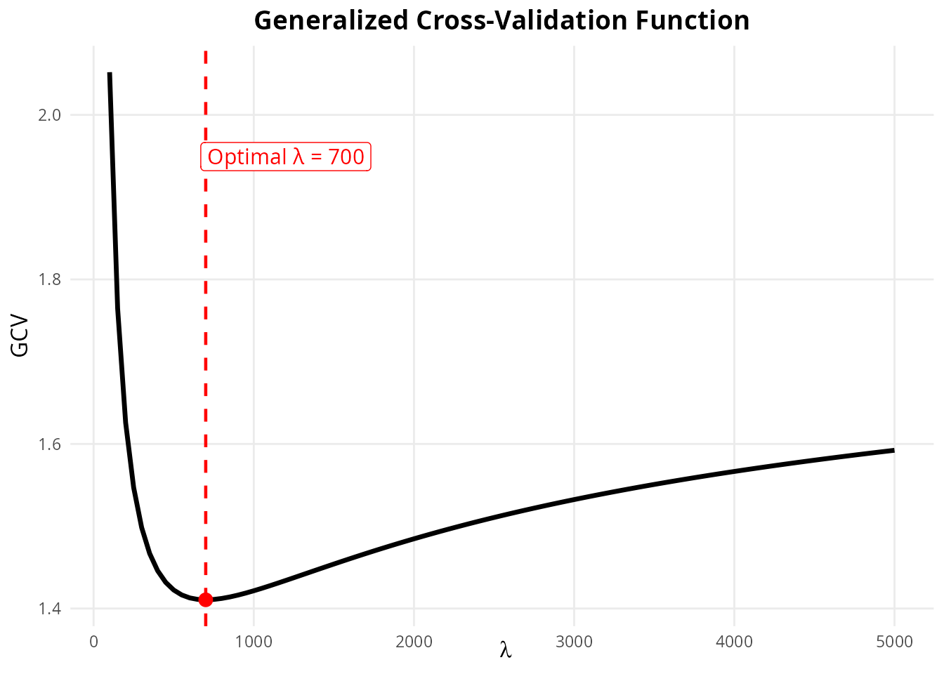
GCV as a Function of Lambda

3. Why Modified HP Filter Works Better

3.1 Simulation Evidence

Choudhary et al. (2014) conducted Monte Carlo simulations comparing the standard HP filter with the Modified HP filter. The data generating process was:

$$g_t = \mu + g_{t-1} + \varepsilon_t, \quad \varepsilon_t \sim N(0, \sigma_\varepsilon^2)$$$$c_t = \phi_1 c_{t-1} + \phi_2 c_{t-2} + \xi_t, \quad \xi_t \sim N(0, \sigma_\xi^2)$$

They varied:

• The ratio $\sigma_\varepsilon / \sigma_\xi$ (relative importance of trend vs cycle)
• AR coefficients $\phi_1, \phi_2$ (cycle persistence)
• Linear vs nonlinear trend specifications

Key finding: The Modified HP filter produced lower mean squared error in recovering the true cycle in nearly 100% of simulations.

set.seed(2024)
n <- 100

# Generate true components
trend_true <- cumsum(c(0, rnorm(n-1, 0.5, 0.2)))
cycle_true <- arima.sim(list(ar = c(1.2, -0.4)), n, sd = 1.5)
y <- trend_true + cycle_true

# Apply both filters
mhp_result <- mhp_filter(y, max_lambda = 10000)
hp_result <- hp_filter(y, lambda = 1600)

# Compute MSE
mse_mhp <- mean((mhp_result$cycle - cycle_true)^2)
mse_hp <- mean((hp_result$cycle - cycle_true)^2)

oldpar <- par(mfrow = c(1, 1))
plot(cycle_true, type = "l", lwd = 2, ylim = range(c(cycle_true, mhp_result$cycle, hp_result$cycle)),
     main = "True vs Estimated Cycles", ylab = "Cycle")
lines(mhp_result$cycle, col = "blue", lwd = 2)
lines(hp_result$cycle, col = "red", lwd = 2, lty = 2)
legend("topright", 
       c(paste0("True Cycle"),
         paste0("MHP (λ=", get_lambda(mhp_result), ", MSE=", round(mse_mhp, 2), ")"),
         paste0("HP (λ=1600, MSE=", round(mse_hp, 2), ")")),
       col = c("black", "blue", "red"), lty = c(1, 1, 2), lwd = 2)

Simulation: True vs Estimated Cycles

par(oldpar)

3.2 Empirical Evidence

Choudhary et al. (2014) estimated optimal $\lambda$ for 93 countries using annual data and 25 countries using quarterly data. Key findings:

Statistic	Annual Data	Quarterly Data
Range of λ	11 - 6,566	229 - 4,898
Fixed λ	100	1,600

Implications:

1. Optimal $\lambda$ varies substantially across countries
2. Few countries have $\lambda$ close to conventional values
3. Standard HP tends to underestimate cyclical volatility (positive sd_diff)
4. AR(1) coefficients are relatively robust to filter choice
5. Correlations between series can differ significantly

# Demonstrate cross-country variation
set.seed(999)

# Simulate countries with different characteristics
countries <- data.table(
  name = c("Stable_Developed", "Volatile_Emerging", "Moderate"),
  trend_sd = c(0.2, 0.5, 0.3),
  cycle_sd = c(0.5, 2.0, 1.0),
  cycle_ar = c(0.9, 0.7, 0.8)
)

results <- lapply(1:nrow(countries), function(i) {
  trend <- cumsum(rnorm(80, 0.5, countries$trend_sd[i]))
  cycle <- arima.sim(list(ar = countries$cycle_ar[i]), 80, sd = countries$cycle_sd[i])
  y <- trend + cycle
  res <- mhp_filter(y, max_lambda = 10000)
  data.table(country = countries$name[i], lambda = get_lambda(res))
})

print(rbindlist(results))
#>              country lambda
#>               <char>  <int>
#> 1:  Stable_Developed    714
#> 2: Volatile_Emerging    604
#> 3:          Moderate    401

4. Theoretical Justification

4.1 Why Cross-Validation?

Cross-validation is optimal in the sense that it asymptotically minimizes the integrated squared error between the estimated trend and the true trend (Craven & Wahba, 1979).

The GCV function has several desirable properties:

1. Rotation invariant: Does not depend on the coordinate system
2. Asymptotically optimal: Converges to the best possible $\lambda$
3. Computationally efficient: Closed-form approximation available

4.2 Relationship to Signal Extraction

The HP filter can be viewed as a Wiener-Kolmogorov filter for signal extraction. If:

• Trend follows a random walk: $\Delta^2 g_t = \varepsilon_t$
• Cycle is stationary noise: $c_t$ stationary

Then $\lambda = \sigma_c^2 / \sigma_\varepsilon^2$ is the optimal filter.

The GCV approach implicitly estimates this ratio from the data.

4.3 Connection to Spline Smoothing

The HP filter is equivalent to a cubic smoothing spline. The GCV method for choosing $\lambda$ is the same used in spline smoothing literature (Silverman, 1984).

5. Practical Recommendations

5.1 When to Use Modified HP Filter

Use Modified HP when:

• Analyzing series from different countries (cross-country comparisons)
• Working with different macro variables (GDP, consumption, investment)
• Unsure about appropriate λ for your specific context
• Need defensible, data-driven parameter selection

Standard HP may be acceptable when:

• Following established literature conventions exactly
• Comparing results with published studies using λ = 1600
• Time series closely matches U.S. quarterly GDP characteristics

5.2 Choosing max_lambda

The max_lambda parameter affects computation time and search range:

max_lambda	Use Case	Speed
5,000	Quick exploratory analysis	~0.05s
10,000	Most quarterly macro series	~0.1s
50,000	Conservative, unusual series	~0.5s
100,000	Very smooth trends needed	~1s

# For most macro applications, 10000 is sufficient
result <- mhp_filter(y, max_lambda = 10000)
cat("Optimal lambda:", get_lambda(result), "\n")
#> Optimal lambda: 1400

# If optimal λ hits the upper bound, increase max_lambda
if (get_lambda(result) >= 9900) {
  warning("Lambda near upper bound - consider increasing max_lambda")
}

5.3 Interpreting Results

Key diagnostics when comparing HP vs Modified HP:

comp <- mhp_compare(y, frequency = "quarterly")
print(comp)
#>         method lambda cycle_sd   cycle_mean       ar1 cycle_range      gcv
#>         <char>  <num>    <num>        <num>     <num>       <num>    <num>
#> 1:          HP   1600 2.444616 1.890115e-12 0.7519842    12.29935       NA
#> 2: Modified HP   1400 2.424745 1.567173e-12 0.7477953    12.20010 6.652109

# Interpretation guide:
# 1. Large lambda difference: series-specific smoothing important
# 2. Positive sd_diff: HP under-estimates cycle volatility
# 3. Large ar1_diff: affects model calibration

6. Mathematical Appendix

6.1 Derivation of HP Filter Solution

The first-order conditions of the minimization problem:

$$\frac{\partial}{\partial g} \left[ (y-g)'(y-g) + \lambda g'A g \right] = 0$$

$$-2(y-g) + 2\lambda A g = 0$$

$$(I + \lambda A)g = y$$

$$g = (I + \lambda A)^{-1} y$$

6.2 Structure of Matrix A

The matrix $A = K'K$ is a symmetric, positive semi-definite band matrix:

$$A = \begin{pmatrix} 1 & -2 & 1 & 0 & 0 & \cdots \\ -2 & 5 & -4 & 1 & 0 & \cdots \\ 1 & -4 & 6 & -4 & 1 & \cdots \\ 0 & 1 & -4 & 6 & -4 & \cdots \\ \vdots & & & \ddots & & \\ \end{pmatrix}$$

This banded structure allows efficient computation using sparse matrix methods (not exploited in this implementation, but potential for future optimization).

6.3 GCV Approximation

Starting from:

$$GCV(\lambda) = \frac{T^{-1} \|y - \hat{g}\|^2}{(1 - T^{-1}\text{tr}(B))^2}$$

Using $(1-x)^{-2} \approx 1 + 2x$ for small $x$:

$$GCV(\lambda) \approx T^{-1} \|y - \hat{g}\|^2 (1 + 2T^{-1}\text{tr}(B))$$

With Silverman’s approximation $\text{tr}(B) \approx T/\lambda$:

$$GCV(\lambda) \approx T^{-1}(1 + 2T/\lambda) \|y - \hat{g}\|^2$$

References

1. Choudhary, M.A., Hanif, M.N., & Iqbal, J. (2014). On smoothing macroeconomic time series using the modified HP filter. Applied Economics, 46(19), 2205-2214.

2. Craven, P., & Wahba, G. (1979). Smoothing noisy data with spline functions. Numerische Mathematik, 31, 377-403.

3. Hodrick, R.J., & Prescott, E.C. (1997). Postwar US business cycles: An empirical investigation. Journal of Money, Credit and Banking, 29(1), 1-16.

4. Marcet, A., & Ravn, M.O. (2004). The HP-filter in cross-country comparisons. CEPR Discussion Paper No. 4244.

5. McDermott, C.J. (1997). An automatic method for choosing the smoothing parameter in the HP filter. Unpublished manuscript, IMF.

6. Ravn, M.O., & Uhlig, H. (2002). On adjusting the Hodrick-Prescott filter for the frequency of observations. Review of Economics and Statistics, 84(2), 371-376.

7. Silverman, B.W. (1984). A fast and efficient cross-validation method for smoothing parameter choice in spline regression. Journal of the American Statistical Association, 79, 584-589.