8  Analysis of Generalized Lattice Designs

8.1 Example 8.1 (Pg. 139)

Example 8.1 (Pg. 139)

In the early 1990s Khongsak Pinyopusarerk of CSIRO Forestry and Forest Products initiated a far-reaching study of Casuarina equisetifolia. This is a nitrogen-fixing tree of considerable social, economic and environmental importance in tropical/subtropical littoral zones of Asia, the Pacific and Africa. Provenance collections were obtained from 18 countries and, with this material, more than 40 trials were laid out in 20 countries. The number of seedlots included in each trial varied, depending on the suitability and size of the planting sites for the available material. One of the trials, in Weipa, northern Queensland, contained all the available seedlots and is the example used here.

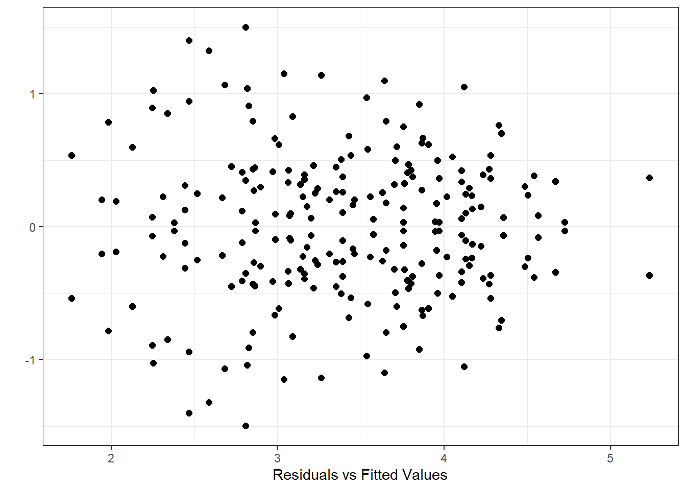
 library(car)

 library(dae)

 library(dplyr)

 library(emmeans)

 library(ggplot2)

 library(lmerTest)

 library(magrittr)

 library(predictmeans)

 data(DataExam8.1)

 # Pg. 141
 fm8.4 <-
   aov(
     formula = dbh ~ inoc + Error(repl/inoc) +
                     inoc*country*prov
   , data    = DataExam8.1
      )

 # Pg. 150
 summary(fm8.4)

Error: repl
          Df Sum Sq Mean Sq F value Pr(>F)  
inoc       1 11.542  11.542   11.46 0.0773 .
Residuals  2  2.014   1.007                 
---
Signif. codes:  0 '***' 0.001 '**' 0.01 '*' 0.05 '.' 0.1 ' ' 1

Error: Within
              Df Sum Sq Mean Sq F value       Pr(>F)    
country       17  54.62   3.213   5.305 0.0000000159 ***
prov          41  18.61   0.454   0.749        0.854    
inoc:country  17  10.07   0.592   0.978        0.487    
inoc:prov     41  21.46   0.523   0.864        0.698    
Residuals    116  70.26   0.606                         
---
Signif. codes:  0 '***' 0.001 '**' 0.01 '*' 0.05 '.' 0.1 ' ' 1

 # Pg. 150
 model.tables(x = fm8.4, type = "means")
Tables of means
Grand mean
        
3.40411 

 inoc 
    7 weeks  1 week
      3.625   3.183
rep 118.000 118.000

 country 
     India Vietnam  Egypt  Kenya   Fiji Thailand Malaysia Philippines Australia
     3.575   3.276  2.498  3.491  2.612    3.841    4.031       3.612     2.631
rep 24.000  20.000 12.000 32.000 12.000   16.000   36.000      12.000    16.000
     PNG Solomon Is. Mauritius Sri Lanka  Guam  China Puerto Rico Vanuatu Benin
    3.65       3.699     3.122     3.243 2.342  3.686       3.345   2.762 3.342
rep 4.00       8.000     4.000    12.000 4.000 12.000       4.000   4.000 4.000

 prov 
        1     2    3    4     5     6     7     8    10    11   12   13    14
    2.623 4.013 3.71 3.27 3.404 3.093 3.701 3.541 3.371 3.301 3.18 3.37 3.404
rep 4.000 4.000 4.00 4.00 4.000 4.000 4.000 4.000 4.000 4.000 4.00 4.00 4.000
       15   16    17    18   19    20    21   22   23    24    25    26   27
    3.595 3.43 3.275 3.085 3.66 3.382 3.235 3.46 3.08 3.555 3.918 3.648 3.43
rep 4.000 4.00 4.000 4.000 4.00 4.000 4.000 4.00 4.00 4.000 4.000 4.000 4.00
       28    29    30    31    32    33    34    35    36    37    38   39   40
    2.905 3.708 3.196 3.761 3.416 3.178 2.958 3.636 3.376 3.404 3.252 3.15 3.81
rep 4.000 4.000 4.000 4.000 4.000 4.000 4.000 4.000 4.000 4.000 4.000 4.00 4.00
       41    42    45   46    47    48    50    51    52    53    54   55    56
    3.195 3.613 3.518 2.76 3.733 3.605 3.404 3.685 3.235 3.755 3.605 2.74 3.662
rep 4.000 4.000 4.000 4.00 4.000 4.000 4.000 4.000 4.000 4.000 4.000 4.00 4.000
       57    58    59    60    61    62    63
    3.408 3.404 3.404 3.528 3.178 3.506 3.418
rep 4.000 4.000 4.000 4.000 4.000 4.000 4.000

 inoc:country 
         country
inoc      India  Vietnam Egypt  Kenya  Fiji   Thailand Malaysia Philippines
  7 weeks  3.672  3.443   2.747  3.609  2.955  3.611    4.502    3.558     
  rep     12.000 10.000   6.000 16.000  6.000  8.000   18.000    6.000     
  1 week   3.477  3.110   2.250  3.373  2.268  4.071    3.559    3.665     
  rep     12.000 10.000   6.000 16.000  6.000  8.000   18.000    6.000     
         country
inoc      Australia PNG    Solomon Is. Mauritius Sri Lanka Guam   China 
  7 weeks  2.959     3.850  4.200       3.390     3.695     2.245  4.030
  rep      8.000     2.000  4.000       2.000     6.000     2.000  6.000
  1 week   2.304     3.450  3.197       2.855     2.792     2.440  3.342
  rep      8.000     2.000  4.000       2.000     6.000     2.000  6.000
         country
inoc      Puerto Rico Vanuatu Benin 
  7 weeks  3.540       2.720   3.870
  rep      2.000       2.000   2.000
  1 week   3.150       2.805   2.815
  rep      2.000       2.000   2.000

 inoc:prov 
         prov
inoc      1     2     3     4     5     6     7     8     10    11    12   
  7 weeks 2.427 4.682 3.757 3.637 3.625 3.540 4.100 3.774 3.559 3.544 3.135
  rep     2.000 2.819 3.344 3.664 2.904 3.183 2.646 3.301 3.308 3.183 3.058
  1 week  2.819 3.344 3.664 2.904 3.183 2.646 3.301 3.308 3.183 3.058 3.225
  rep     2.427 4.682 3.757 3.637 3.625 3.540 4.100 3.774 3.559 3.544 3.135
         prov
inoc      13    14    15    16    17    18    19    20    21    22    23   
  7 weeks 3.845 3.625 4.104 4.119 3.604 3.114 3.509 3.304 3.591 3.801 3.276
  rep     3.225 2.895 3.183 3.085 2.740 2.945 3.055 3.810 3.460 2.880 3.120
  1 week  2.895 3.183 3.085 2.740 2.945 3.055 3.810 3.460 2.880 3.120 2.885
  rep     3.845 3.625 4.104 4.119 3.604 3.114 3.509 3.304 3.591 3.801 3.276
         prov
inoc      24    25    26    27    28    29    30    31    32    33    34   
  7 weeks 3.021 3.976 4.286 4.186 2.866 3.663 2.988 3.793 4.358 3.343 3.468
  rep     2.885 4.090 3.860 3.010 2.675 2.945 3.754 3.404 3.729 2.474 3.014
  1 week  4.090 3.860 3.010 2.675 2.945 3.754 3.404 3.729 2.474 3.014 2.449
  rep     3.021 3.976 4.286 4.186 2.866 3.663 2.988 3.793 4.358 3.343 3.468
         prov
inoc      35    36    37    38    39    40    41    42    45    46    47   
  7 weeks 3.848 3.688 3.625 3.772 3.132 3.972 3.545 3.705 3.439 2.599 4.119
  rep     2.449 3.424 3.064 3.183 2.733 3.168 3.648 2.845 3.520 3.597 2.922
  1 week  3.424 3.064 3.183 2.733 3.168 3.648 2.845 3.520 3.597 2.922 3.347
  rep     3.848 3.688 3.625 3.772 3.132 3.972 3.545 3.705 3.439 2.599 4.119
         prov
inoc      48    50    51    52    53    54    55    56    57    58    59   
  7 weeks 4.344 3.625 4.137 4.152 4.047 3.167 2.622 3.895 3.478 3.625 3.625
  rep     3.347 2.867 3.183 3.233 2.318 3.463 4.043 2.858 3.430 3.339 3.183
  1 week  2.867 3.183 3.233 2.318 3.463 4.043 2.858 3.430 3.339 3.183 3.183
  rep     4.344 3.625 4.137 4.152 4.047 3.167 2.622 3.895 3.478 3.625 3.625
         prov
inoc      60    61    62    63   
  7 weeks 3.685 3.630 3.560 3.235
  rep     3.183 3.371 2.726 3.451
  1 week  3.371 2.726 3.451 3.601
  rep     3.685 3.630 3.560 3.235

 RESFit <-
     data.frame(
       fittedvalue   = fitted.aovlist(fm8.4)
     , residualvalue = proj(fm8.4)$Within[,"Residuals"]
     )

 ggplot(
    data    =  RESFit
  , mapping = aes(x = fittedvalue, y = residualvalue)
  ) +
 geom_point(size = 2) +
 labs(
    x = "Residuals vs Fitted Values"
  , y = ""
  ) +
 theme_bw()

 # Pg. 153
 fm8.6 <-
  aov(
    formula = terms(
                    dbh ~ inoc + repl + col +
                          repl:row + repl:col +
                          prov + inoc:prov
                    , keep.order = TRUE
                    )
  , data   = DataExam8.1
  )

 summary(fm8.6)
            Df Sum Sq Mean Sq F value               Pr(>F)    
inoc         1  11.54  11.542  48.054        0.00000000327 ***
repl         2   2.01   1.007   4.193             0.019746 *  
col          9  65.24   7.249  30.182 < 0.0000000000000002 ***
repl:row    20  16.59   0.830   3.454             0.000105 ***
repl:col    27  16.41   0.608   2.530             0.001443 ** 
prov        58  53.89   0.929   3.869        0.00000026687 ***
inoc:prov   58   8.47   0.146   0.608             0.970544    
Residuals   60  14.41   0.240                                 
---
Signif. codes:  0 '***' 0.001 '**' 0.01 '*' 0.05 '.' 0.1 ' ' 1

8.2 Example 8.1 (continued) (Pg. 147)

Example 8.1 (continued) (Pg. 147)

 library(car)

 library(dae)

 library(dplyr)

 library(emmeans)

 library(ggplot2)

 library(lmerTest)

 library(magrittr)

 library(predictmeans)

 data(DataExam8.1)

 # Pg. 155
 fm8.8 <-
  lmerTest::lmer(
      formula = dbh ~ 1 + repl + col + prov +
                      (1|repl:row) + (1|repl:col)
    , data   = DataExam8.1
    , REML   = TRUE
    )

 # Pg. 157
 #\dontrun{
 varcomp(fm8.8)
                       vcov     SE  2.5 % 97.5 %
repl:col.(Intercept) 0.0459 0.0262 0.0000 0.0565
repl:row.(Intercept) 0.0640 0.0294 0.0210 0.1161
residual             0.1951 0.0253 0.1126 0.1782

 #}
 
 anova(fm8.8)
Type III Analysis of Variance Table with Satterthwaite's method
     Sum Sq Mean Sq NumDF   DenDF F value              Pr(>F)    
repl  2.581 0.86023     3  21.257  4.4082             0.01469 *  
col  24.874 2.76378     9  23.705 14.1627 0.00000015112494790 ***
prov 55.433 0.95574    58 136.623  4.8976 0.00000000000001306 ***
---
Signif. codes:  0 '***' 0.001 '**' 0.01 '*' 0.05 '.' 0.1 ' ' 1

 anova(fm8.8, ddf = "Kenward-Roger")
Type III Analysis of Variance Table with Kenward-Roger's method
     Sum Sq Mean Sq NumDF   DenDF F value             Pr(>F)    
repl  2.580 0.86016     3  22.622  4.4078             0.0139 *  
col  24.824 2.75827     9  22.947 14.1337 0.0000002097637857 ***
prov 54.795 0.94473    58 133.852  4.8396 0.0000000000000283 ***
---
Signif. codes:  0 '***' 0.001 '**' 0.01 '*' 0.05 '.' 0.1 ' ' 1

 predictmeans(model = fm8.8, modelterm = "repl")

$`Predicted Means`
repl
     1      2      3      4 
3.7543 3.1269 3.2128 3.5023 

$`Standard Error of Means`
All means have the same SE 
                   0.13629 

$`Standard Error of Differences`
  Max.SED   Min.SED  Aveg.SED 
0.1927495 0.1927423 0.1927472 

$LSD
 Max.LSD  Min.LSD Aveg.LSD 
 0.39910  0.39909  0.39910 
attr(,"Significant level")
[1] 0.05
attr(,"Degree of freedom")
[1] 22.62

$mean_table
  repl   Mean      SE      Df LL(95%) UL(95%)
1    1 3.7543 0.13629 22.6214  3.4721  4.0365
2    2 3.1269 0.13629 22.6214  2.8447  3.4091
3    3 3.2128 0.13629 22.6214  2.9306  3.4950
4    4 3.5023 0.13629 22.6214  3.2201  3.7845


 predictmeans(model = fm8.8, modelterm = "col")

$`Predicted Means`
col
     1      2      3      4      5      6      7      8      9     10 
3.5053 3.4996 3.8509 3.8280 3.5947 3.7829 3.3059 3.5158 3.1776 1.9301 

$`Standard Error of Means`
col
      1       2       3       4       5       6       7       8       9      10 
0.15496 0.15649 0.15493 0.15494 0.15490 0.15721 0.15479 0.15699 0.15485 0.15648 

$`Standard Error of Differences`
  Max.SED   Min.SED  Aveg.SED 
0.2132295 0.2061223 0.2086161 

$LSD
 Max.LSD  Min.LSD Aveg.LSD 
 0.43742  0.42284  0.42796 
attr(,"Significant level")
[1] 0.05
attr(,"Degree of freedom")
[1] 27.12

$mean_table
   col   Mean      SE       Df LL(95%) UL(95%)
1    1 3.5053 0.15496 27.11736  3.1874  3.8232
2    2 3.4996 0.15649 27.11736  3.1786  3.8207
3    3 3.8509 0.15493 27.11736  3.5330  4.1687
4    4 3.8280 0.15494 27.11736  3.5101  4.1458
5    5 3.5947 0.15490 27.11736  3.2769  3.9125
6    6 3.7829 0.15721 27.11736  3.4604  4.1054
7    7 3.3059 0.15479 27.11736  2.9883  3.6234
8    8 3.5158 0.15699 27.11736  3.1938  3.8379
9    9 3.1776 0.15485 27.11736  2.8599  3.4952
10  10 1.9301 0.15648 27.11736  1.6091  2.2511


 predictmeans(model = fm8.8, modelterm = "prov")

$`Predicted Means`
prov
     1      2      3      4      5      6      7      8     10     11     12 
2.4222 3.1425 2.8646 2.2599 3.7189 3.5445 3.9474 2.7469 2.6459 2.0497 2.7497 
    13     14     15     16     17     18     19     20     21     22     23 
2.9833 2.6534 3.4459 3.9209 3.4294 3.3624 3.6540 3.3685 3.2210 3.3315 3.2453 
    24     25     26     27     28     29     30     31     32     33     34 
3.6933 3.8460 3.5233 3.5271 3.1001 3.8997 3.5447 4.1294 4.2755 3.7429 3.8890 
    35     36     37     38     39     40     41     42     45     46     47 
4.1179 3.8526 3.4538 3.0379 3.5306 3.7412 3.7422 3.8765 4.2126 3.4660 4.4688 
    48     50     51     52     53     54     55     56     57     58     59 
3.7503 2.5571 3.4571 3.3227 3.5926 3.5337 2.7157 2.7702 3.9805 2.9968 3.3978 
    60     61     62     63 
3.0115 3.2238 3.2814 3.5751 

$`Standard Error of Means`
prov
      1       2       3       4       5       6       7       8      10      11 
0.25362 0.25446 0.25278 0.25443 0.25423 0.25588 0.25420 0.25338 0.25417 0.25259 
     12      13      14      15      16      17      18      19      20      21 
0.25306 0.25436 0.25259 0.25232 0.25502 0.25319 0.25340 0.25309 0.25294 0.25204 
     22      23      24      25      26      27      28      29      30      31 
0.25350 0.25355 0.25358 0.25316 0.25289 0.25294 0.25291 0.25341 0.25254 0.25330 
     32      33      34      35      36      37      38      39      40      41 
0.25377 0.25387 0.25510 0.25347 0.25351 0.25352 0.25416 0.25393 0.25450 0.25416 
     42      45      46      47      48      50      51      52      53      54 
0.25303 0.25257 0.25323 0.25316 0.25356 0.25354 0.25372 0.25361 0.25237 0.25321 
     55      56      57      58      59      60      61      62      63 
0.25374 0.25639 0.25173 0.25319 0.25250 0.25303 0.25378 0.25266 0.25500 

$`Standard Error of Differences`
  Max.SED   Min.SED  Aveg.SED 
0.3591712 0.3326719 0.3482665 

$LSD
 Max.LSD  Min.LSD Aveg.LSD 
 0.70924  0.65691  0.68770 
attr(,"Significant level")
[1] 0.05
attr(,"Degree of freedom")
[1] 162.73

$mean_table
   prov   Mean      SE       Df LL(95%) UL(95%)
1     1 2.4222 0.25362 162.7269  1.9214  2.9230
2     2 3.1425 0.25446 162.7269  2.6401  3.6450
3     3 2.8646 0.25278 162.7269  2.3655  3.3638
4     4 2.2599 0.25443 162.7269  1.7575  2.7623
5     5 3.7189 0.25423 162.7269  3.2169  4.2209
6     6 3.5445 0.25588 162.7269  3.0392  4.0498
7     7 3.9474 0.25420 162.7269  3.4454  4.4493
8     8 2.7469 0.25338 162.7269  2.2466  3.2473
9    10 2.6459 0.25417 162.7269  2.1440  3.1478
10   11 2.0497 0.25259 162.7269  1.5509  2.5485
11   12 2.7497 0.25306 162.7269  2.2500  3.2494
12   13 2.9833 0.25436 162.7269  2.4810  3.4855
13   14 2.6534 0.25259 162.7269  2.1546  3.1522
14   15 3.4459 0.25232 162.7269  2.9476  3.9441
15   16 3.9209 0.25502 162.7269  3.4173  4.4245
16   17 3.4294 0.25319 162.7269  2.9294  3.9293
17   18 3.3624 0.25340 162.7269  2.8620  3.8628
18   19 3.6540 0.25309 162.7269  3.1543  4.1538
19   20 3.3685 0.25294 162.7269  2.8690  3.8680
20   21 3.2210 0.25204 162.7269  2.7234  3.7187
21   22 3.3315 0.25350 162.7269  2.8310  3.8321
22   23 3.2453 0.25355 162.7269  2.7447  3.7460
23   24 3.6933 0.25358 162.7269  3.1926  4.1941
24   25 3.8460 0.25316 162.7269  3.3461  4.3459
25   26 3.5233 0.25289 162.7269  3.0239  4.0227
26   27 3.5271 0.25294 162.7269  3.0276  4.0265
27   28 3.1001 0.25291 162.7269  2.6007  3.5996
28   29 3.8997 0.25341 162.7269  3.3993  4.4001
29   30 3.5447 0.25254 162.7269  3.0460  4.0434
30   31 4.1294 0.25330 162.7269  3.6293  4.6296
31   32 4.2755 0.25377 162.7269  3.7744  4.7766
32   33 3.7429 0.25387 162.7269  3.2416  4.2442
33   34 3.8890 0.25510 162.7269  3.3853  4.3928
34   35 4.1179 0.25347 162.7269  3.6174  4.6185
35   36 3.8526 0.25351 162.7269  3.3520  4.3532
36   37 3.4538 0.25352 162.7269  2.9532  3.9544
37   38 3.0379 0.25416 162.7269  2.5360  3.5398
38   39 3.5306 0.25393 162.7269  3.0291  4.0320
39   40 3.7412 0.25450 162.7269  3.2386  4.2437
40   41 3.7422 0.25416 162.7269  3.2403  4.2440
41   42 3.8765 0.25303 162.7269  3.3769  4.3761
42   45 4.2126 0.25257 162.7269  3.7139  4.7114
43   46 3.4660 0.25323 162.7269  2.9660  3.9661
44   47 4.4688 0.25316 162.7269  3.9689  4.9687
45   48 3.7503 0.25356 162.7269  3.2496  4.2510
46   50 2.5571 0.25354 162.7269  2.0564  3.0577
47   51 3.4571 0.25372 162.7269  2.9561  3.9582
48   52 3.3227 0.25361 162.7269  2.8219  3.8235
49   53 3.5926 0.25237 162.7269  3.0943  4.0910
50   54 3.5337 0.25321 162.7269  3.0337  4.0337
51   55 2.7157 0.25374 162.7269  2.2146  3.2167
52   56 2.7702 0.25639 162.7269  2.2640  3.2765
53   57 3.9805 0.25173 162.7269  3.4834  4.4776
54   58 2.9968 0.25319 162.7269  2.4968  3.4968
55   59 3.3978 0.25250 162.7269  2.8992  3.8963
56   60 3.0115 0.25303 162.7269  2.5118  3.5112
57   61 3.2238 0.25378 162.7269  2.7227  3.7250
58   62 3.2814 0.25266 162.7269  2.7825  3.7803
59   63 3.5751 0.25500 162.7269  3.0716  4.0787


  # Pg. 161
   RCB1 <-
         aov(dbh ~ prov + repl, data = DataExam8.1)

   RCB  <-
         emmeans(RCB1,  specs = "prov") %>%
         as_tibble()

   Mixed <-
           emmeans(fm8.8, specs = "prov") %>%
           as_tibble()

   table8.9 <-
       left_join(
          x      = RCB
        , y      = Mixed
        , by     = "prov"
        , suffix = c(".RCBD", ".Mixed")
        )

   print(table8.9)
# A tibble: 59 × 11
   prov  emmean.RCBD SE.RCBD df.RCBD lower.CL.RCBD upper.CL.RCBD emmean.Mixed
   <fct>       <dbl>   <dbl>   <dbl>         <dbl>         <dbl>        <dbl>
 1 1            1.85   0.382     174          1.10          2.60         2.42
 2 2            3.24   0.382     174          2.49          3.99         3.14
 3 3            2.94   0.382     174          2.18          3.69         2.86
 4 4            2.50   0.382     174          1.74          3.25         2.26
 5 5            3.34   0.382     174          2.59          4.10         3.72
 6 6            3.37   0.382     174          2.62          4.13         3.54
 7 7            3.98   0.382     174          3.23          4.74         3.95
 8 8            2.63   0.382     174          1.88          3.39         2.75
 9 10           2.47   0.382     174          1.71          3.22         2.65
10 11           2.40   0.382     174          1.64          3.15         2.05
# ℹ 49 more rows
# ℹ 4 more variables: SE.Mixed <dbl>, df.Mixed <dbl>, lower.CL.Mixed <dbl>,
#   upper.CL.Mixed <dbl>

8.3 Example 8.1 (continued) (Pg. 155)

Example 8.1 (continued) (Pg. 155)

 library(car)

 library(dae)

 library(dplyr)

 library(emmeans)

 library(ggplot2)

 library(lmerTest)

 library(magrittr)

 library(predictmeans)

 data(DataExam8.1)

 # Pg. 167
 fm8.11 <-
   aov(
        formula = dbh ~ country + country:prov
      , data    = DataExam8.1
       )

   b <- anova(fm8.11)

   Res <- length(b[["Sum Sq"]])

   df  <- 119

   MSS <- 0.1951

   b[["Df"]][Res] <- df

   b[["Sum Sq"]][Res] <- MSS*df

   b[["Mean Sq"]][Res] <- b[["Sum Sq"]][Res]/b[["Df"]][Res]

   b[["F value"]][1:Res-1] <-
             b[["Mean Sq"]][1:Res-1]/b[["Mean Sq"]][Res]

   b[["Pr(>F)"]][Res-1] <-
      df(
        b[["F value"]][Res-1]
      , b[["Df"]][Res-1]
      , b[["Df"]][Res]
      )

   b
Analysis of Variance Table

Response: dbh
              Df Sum Sq Mean Sq F value        Pr(>F)    
country       17 54.619  3.2129  16.468 0.00000001235 ***
country:prov  41 18.606  0.4538   2.326      0.001502 ** 
Residuals    119 23.217  0.1951                          
---
Signif. codes:  0 '***' 0.001 '**' 0.01 '*' 0.05 '.' 0.1 ' ' 1

  emmeans(fm8.11, specs = "country")
 country     emmean    SE  df lower.CL upper.CL
 India         3.57 0.165 177     3.25     3.90
 Vietnam       3.28 0.181 177     2.92     3.63
 Egypt         2.50 0.233 177     2.04     2.96
 Kenya         3.49 0.143 177     3.21     3.77
 Fiji          2.61 0.233 177     2.15     3.07
 Thailand      3.84 0.202 177     3.44     4.24
 Malaysia      4.03 0.135 177     3.77     4.30
 Philippines   3.61 0.233 177     3.15     4.07
 Australia     2.63 0.202 177     2.23     3.03
 PNG           3.65 0.404 177     2.85     4.45
 Solomon Is.   3.70 0.285 177     3.14     4.26
 Mauritius     3.12 0.404 177     2.33     3.92
 Sri Lanka     3.24 0.233 177     2.78     3.70
 Guam          2.34 0.404 177     1.55     3.14
 China         3.69 0.233 177     3.23     4.15
 Puerto Rico   3.35 0.404 177     2.55     4.14
 Vanuatu       2.76 0.404 177     1.97     3.56
 Benin         3.34 0.404 177     2.55     4.14

Results are averaged over the levels of: prov 
Confidence level used: 0.95 

8.4 Example 8.2 (Pg. 157)

Example 8.2 (Pg. 157)

In Example 7.1 we discussed a Eucalyptus clone trial conducted in Vietnam and described the experimental layout. The trial tested 56 hybrid clones of the interspecific hybrid combination E. urophylla \(\times\) E. pellita (UP). These candidates had been selected from progeny trials of control-pollinated hybrid families; here we ignore the parental origins of the different UP clones.

 library(car)

 library(dae)

 library(dplyr)

 library(emmeans)

 library(ggplot2)

 library(lmerTest)

 library(magrittr)

 library(predictmeans)

 data(DataExam8.2)

 # Pg.
 fm8.2  <-
   lmerTest::lmer(
     formula = dbh ~ repl + column +
                     contcompf + contcompf:standard +
                     (1|repl:row) + (1|repl:column) +
                     (1|contcompv:clone)
   , data    = DataExam8.2
     )

 #\dontrun{
 varcomp(fm8.2)
                              vcov     SE  2.5 % 97.5 %
contcompv:clone.(Intercept) 0.4950 0.1126 0.3057 0.7422
repl:row.(Intercept)        0.0802 0.0351 0.0173 0.1458
repl:column.(Intercept)     0.0529 0.0326 0.0000 0.0783
residual                    0.3992 0.0435 0.3245 0.5024

 #}
 anova(fm8.2)
Type III Analysis of Variance Table with Satterthwaite's method
                    Sum Sq Mean Sq NumDF   DenDF F value          Pr(>F)    
repl                3.2720  0.8180     4  26.467  2.0489       0.1162606    
column              3.1018  0.6204     5  19.545  1.5539       0.2194719    
contcompf           5.3203  5.3203     1  54.905 13.3265       0.0005845 ***
contcompf:standard 20.6587  6.8862     3 207.152 17.2488 0.0000000004896 ***
---
Signif. codes:  0 '***' 0.001 '**' 0.01 '*' 0.05 '.' 0.1 ' ' 1

 Anova(fm8.2, type = "II", test.statistic = "Chisq")
Analysis of Deviance Table (Type II Wald chisquare tests)

Response: dbh
                     Chisq Df Pr(>Chisq)    
repl                8.1957  4    0.08467 .  
column              7.7694  5    0.16941    
contcompf           4.6841  1    0.03044 *  
contcompf:standard 51.7463  3  3.392e-11 ***
---
Signif. codes:  0 '***' 0.001 '**' 0.01 '*' 0.05 '.' 0.1 ' ' 1

 predictmeans(model = fm8.2, modelterm = "repl")

$`Predicted Means`
repl
     1      2      3      4      5 
7.8926 8.2070 8.3429 8.4604 8.5464 

$`Standard Error of Means`
repl
      1       2       3       4       5 
0.33123 0.33126 0.32992 0.32992 0.32992 

$`Standard Error of Differences`
  Max.SED   Min.SED  Aveg.SED 
0.2239675 0.2167320 0.2196681 

$LSD
 Max.LSD  Min.LSD Aveg.LSD 
 0.44792  0.43345  0.43932 
attr(,"Significant level")
[1] 0.05
attr(,"Degree of freedom")
[1] 60.56

$mean_table
  repl   Mean      SE       Df LL(95%) UL(95%)
1    1 7.8926 0.33123 60.55892  7.2302  8.5551
2    2 8.2070 0.33126 60.55892  7.5445  8.8695
3    3 8.3429 0.32992 60.55892  7.6831  9.0027
4    4 8.4604 0.32992 60.55892  7.8006  9.1202
5    5 8.5464 0.32992 60.55892  7.8866  9.2062


 predictmeans(model = fm8.2, modelterm = "column")

$`Predicted Means`
column
     1      2      3      4      5      6 
8.2214 8.4708 8.3779 7.9721 7.8166 8.7141 

$`Standard Error of Means`
column
      1       2       3       4       5       6 
0.31662 0.39168 0.39315 0.26648 0.26646 0.31653 

$`Standard Error of Differences`
  Max.SED   Min.SED  Aveg.SED 
0.2714760 0.2102583 0.2373610 

$LSD
 Max.LSD  Min.LSD Aveg.LSD 
 0.54250  0.42017  0.47433 
attr(,"Significant level")
[1] 0.05
attr(,"Degree of freedom")
[1] 62.99

$mean_table
  column   Mean      SE       Df LL(95%) UL(95%)
1      1 8.2214 0.31662 62.99437  7.5887  8.8542
2      2 8.4708 0.39168 62.99437  7.6881  9.2535
3      3 8.3779 0.39315 62.99437  7.5923  9.1636
4      4 7.9721 0.26648 62.99437  7.4396  8.5047
5      5 7.8166 0.26646 62.99437  7.2841  8.3491
6      6 8.7141 0.31653 62.99437  8.0816  9.3467


 emmeans(object = fm8.2, specs = ~contcompf|standard)
contcompf = 1, standard = 0:
 emmean    SE   df lower.CL upper.CL
   8.91 0.117 65.9     8.67     9.14

contcompf = 0, standard = UG323:
 emmean    SE   df lower.CL upper.CL
   8.97 0.770 55.6     7.43    10.51

contcompf = 0, standard = U6:
 emmean    SE   df lower.CL upper.CL
   6.55 0.770 55.5     5.01     8.10

contcompf = 0, standard = PN14:
 emmean    SE   df lower.CL upper.CL
   7.70 0.771 55.8     6.16     9.25

contcompf = 0, standard = SSOseed:
 emmean    SE   df lower.CL upper.CL
   6.08 0.770 55.5     4.54     7.63

Results are averaged over the levels of: repl, column 
Degrees-of-freedom method: kenward-roger 
Confidence level used: 0.95