3  Data Collection and Pre-Processing

3.1 Example 3.1 (Pg. 30)

Example 3.1 (Pg. 30)

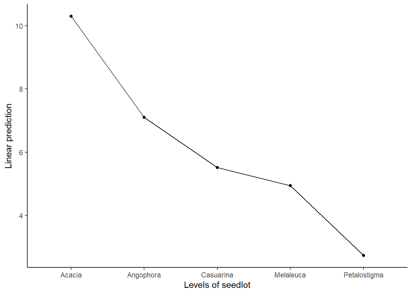
We illustrate the recommended layout for data sheets with one of the trials conducted by the Australian Centre for International Agricultural Research (ACIAR) in Queensland, Australia (Experiment 309). This was a species trial planted in 1985; survival was poor. For our example we will examine only part of the data from this experiment. Five of the species with good survival have been extracted at random, namely Acacia, Angophora, Casuarina, Melaleuca and Petalostigma.

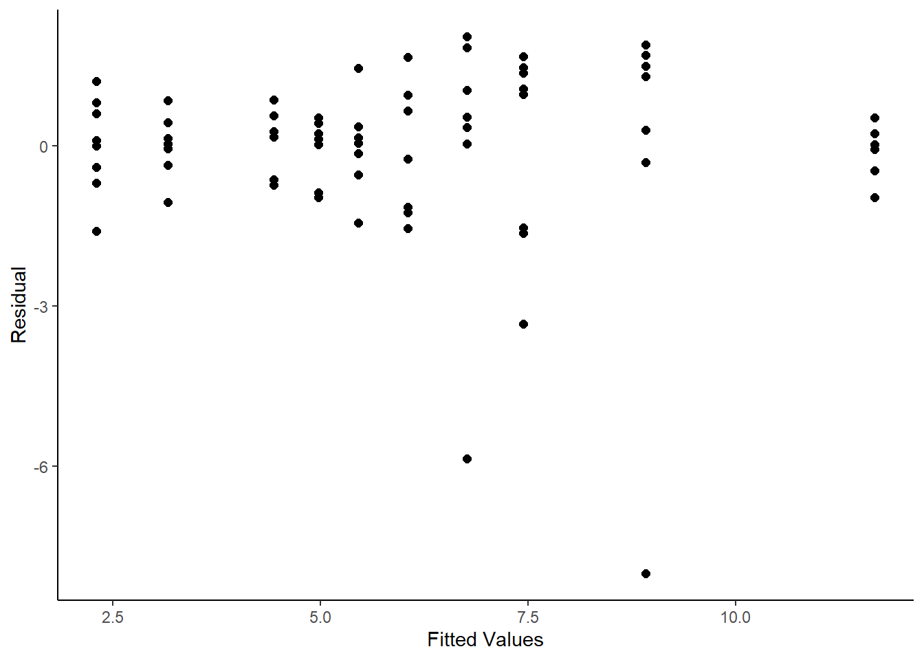
 library(car)

 library(dae)

 library(dplyr)

 library(emmeans)

 library(ggplot2)

 library(lmerTest)

 library(magrittr)

 library(predictmeans)

 library(supernova)

 data(DataExam3.1)

 # Pg. 28
 fmtab3.3 <-
           lm(
               formula = ht ~ repl*seedlot
             , data    = DataExam3.1
             )

 fmtab3.3ANOVA1 <-
   anova(fmtab3.3) %>%
   mutate(
   "F value" =
          c(
            anova(fmtab3.3)[1:2, 3]/anova(fmtab3.3)[3, 3]
          , anova(fmtab3.3)[3, 4]
          , NA
          )
           )

  # Pg. 33 (Table 3.3)
 fmtab3.3ANOVA1 %>%
   mutate(
   "Pr(>F)"  =
        c(
          NA
        , pf(
             q   = fmtab3.3ANOVA1[2, 4]
           , df1 = fmtab3.3ANOVA1[2, 1]
           , df2 = fmtab3.3ANOVA1[3, 1], lower.tail = FALSE
           )
        , NA
        , NA
        )
        )
             Df Sum Sq Mean Sq F value   Pr(>F)   
repl          1  20.30  20.301  3.4197            
seedlot       4 505.87 126.467 21.3035 0.005851 **
repl:seedlot  4  23.75   5.936  2.3663            
Residuals    70 175.61   2.509                    
---
Signif. codes:  0 '***' 0.001 '**' 0.01 '*' 0.05 '.' 0.1 ' ' 1

  # Pg. 33  (Table 3.3)
  emmeans(object  = fmtab3.3, specs = ~ seedlot)
 seedlot      emmean    SE df lower.CL upper.CL
 Acacia        10.29 0.396 70     9.50    11.08
 Angophora      7.10 0.396 70     6.31     7.89
 Casuarina      5.51 0.396 70     4.72     6.30
 Melaleuca      4.94 0.396 70     4.15     5.73
 Petalostigma   2.73 0.396 70     1.94     3.52

Results are averaged over the levels of: repl 
Confidence level used: 0.95 

  # Pg. 34  (Figure 3.2)
  ggplot(
     mapping = aes(
                   x = fitted.values(fmtab3.3)
                 , y = residuals(fmtab3.3)
                 )
                 ) +
  geom_point(size = 2) +
  labs(
     x = "Fitted Values"
   , y = "Residual"
    ) +
  theme_classic()

 # Pg. 33 (Table 3.4)
 DataExam3.1m <- DataExam3.1

 DataExam3.1m[c(28, 51, 76), 5] <- NA

 DataExam3.1m[c(28, 51, 76), 6] <- NA

 fmtab3.4 <-
           lm(
               formula   = ht ~ repl*seedlot
             , data      = DataExam3.1m
             )

 fmtab3.4ANOVA1 <-
   anova(fmtab3.4) %>%
   mutate(
       "F value" =
             c(
                anova(fmtab3.4)[1:2, 3]/anova(fmtab3.4)[3, 3]
              , anova(fmtab3.4)[3, 4]
              , NA
              )
              )

 # Pg. 33 (Table 3.4)
 fmtab3.4ANOVA1 %>%
   mutate(
   "Pr(>F)"  =
        c(
          NA
        , pf(
             q   = fmtab3.4ANOVA1[2, 4]
           , df1 = fmtab3.4ANOVA1[2, 1]
           , df2 = fmtab3.4ANOVA1[3, 1], lower.tail = FALSE
           )
        , NA
        , NA
        )
        )
             Df Sum Sq Mean Sq F value  Pr(>F)    
repl          1  18.88  18.877 10.4201            
seedlot       4 588.68 147.169 81.2367 0.00044 ***
repl:seedlot  4   7.25   1.812  2.4163            
Residuals    67  50.23   0.750                    
---
Signif. codes:  0 '***' 0.001 '**' 0.01 '*' 0.05 '.' 0.1 ' ' 1

  # Pg. 33  (Table 3.4)
  emmeans(object  = fmtab3.4, specs = ~ seedlot)
 seedlot      emmean    SE df lower.CL upper.CL
 Acacia        10.87 0.224 67    10.42    11.31
 Angophora      7.76 0.231 67     7.30     8.22
 Casuarina      5.51 0.216 67     5.08     5.94
 Melaleuca      4.94 0.216 67     4.51     5.38
 Petalostigma   2.73 0.216 67     2.30     3.16

Results are averaged over the levels of: repl 
Confidence level used: 0.95 

3.2 Example 3.1 (continued) (Pg. 34)

Example 3.1 (continued) (Pg. 34)

The analysis of variance table for ht is given below:

 library(car)

 library(dae)

 library(dplyr)

 library(emmeans)

 library(ggplot2)

 library(lmerTest)

 library(magrittr)

 library(predictmeans)

 data(DataExam3.1.1)

 # Pg. 36
 fm3.8 <-
       lm(
          formula = ht ~ repl + seedlot
        , data    = DataExam3.1.1
        )

 # Pg. 40
 anova(fm3.8)
Analysis of Variance Table

Response: ht
          Df Sum Sq Mean Sq F value   Pr(>F)   
repl       1  2.538  2.5376  3.4197 0.138108   
seedlot    4 63.234 15.8084 21.3035 0.005851 **
Residuals  4  2.968  0.7421                    
---
Signif. codes:  0 '***' 0.001 '**' 0.01 '*' 0.05 '.' 0.1 ' ' 1

 # Pg. 40
 emmeans(object = fm3.8, specs  = ~seedlot)
 seedlot      emmean    SE df lower.CL upper.CL
 Acacia        10.29 0.609  4     8.60    11.98
 Angophora      7.10 0.609  4     5.41     8.79
 Casuarina      5.51 0.609  4     3.82     7.20
 Melaleuca      4.94 0.609  4     3.25     6.63
 Petalostigma   2.73 0.609  4     1.04     4.42

Results are averaged over the levels of: repl 
Confidence level used: 0.95 

 emmip(object = fm3.8, formula  = ~seedlot) +
  theme_classic()