4  Experimental Design

4.1 Example 4.3 (Pg. 53)

Example 4.3 (Pg. 53)

Major seed distributors such as the Australian Tree Seed Centre (ATSC) routinely conduct seed viability tests so that, when seed is dispatched, the purchaser has an indication of the germination percentage of the seed. As part of the ATSC research program, a series of experiments was conducted in 1992 by Debbie Solomon on provenances of Acacia mangium to investigate methods of pre-treatment and loss of viability of stored seed. Each experiment involved six seedlots of Acacia mangium and four seed pre-treatments in a factorial design with three replicates.

 library(car)

 library(dae)

 library(dplyr)

 library(emmeans)

 library(ggplot2)

 library(lmerTest)

 library(magrittr)

 library(predictmeans)

 data(DataExam4.3)

  # Pg. 50
  fm4.2    <-
    aov(
        formula =
        percent ~ repl + contcomp + seedlot +
                  treat/contcomp + contcomp/seedlot +
                  treat/contcomp/seedlot
       , data   = DataExam4.3
      )

  # Pg. 54
  anova(fm4.2)
Analysis of Variance Table

Response: percent
                       Df Sum Sq Mean Sq  F value                Pr(>F)    
repl                    2     35      18   0.1804             0.8355379    
contcomp                1  58542   58542 601.5217 < 0.00000000000000022 ***
seedlot                 5   2894     579   5.9481             0.0002538 ***
treat                   2   5300    2650  27.2295         0.00000001576 ***
contcomp:seedlot        5   1347     269   2.7682             0.0287571 *  
contcomp:seedlot:treat 10    961      96   0.9876             0.4674993    
Residuals              46   4477      97                                   
---
Signif. codes:  0 '***' 0.001 '**' 0.01 '*' 0.05 '.' 0.1 ' ' 1

  # Pg. 54
  model.tables(x = fm4.2, type = "means")
Tables of means
Grand mean
         
51.38889 

 repl 
        1     2     3
    52.33 50.67 51.17
rep 24.00 24.00 24.00

 contcomp 
    Treated control
      67.85       2
rep   54.00      18

 seedlot 
    18211 18212 18217 18248 18249 18265
       58 52.33    49 40.67 48.67 59.67
rep    12 12.00    12 12.00 12.00 12.00

 treat 
     nick  bw&s control bw1min
    40.43 49.31   51.39  64.43
rep 18.00 18.00   18.00  18.00

 contcomp:seedlot 
         seedlot
contcomp  18211 18212 18217 18248 18249 18265
  Treated 77.33 69.33 63.11 53.33 64.89 79.11
  rep      9.00  9.00  9.00  9.00  9.00  9.00
  control  0.00  1.33  6.67  2.67  0.00  1.33
  rep      3.00  3.00  3.00  3.00  3.00  3.00

 contcomp:seedlot:treat 
, , treat = nick

         seedlot
contcomp  18211 18212 18217 18248 18249 18265
  Treated 65.33 54.67 57.33 40.00 49.33 74.67
  rep      3.00  3.00  3.00  3.00  3.00  3.00
  control                                    
  rep      0.00  0.00  0.00  0.00  0.00  0.00

, , treat = bw&s

         seedlot
contcomp  18211 18212 18217 18248 18249 18265
  Treated 78.67 68.00 54.67 52.00 61.33 80.00
  rep      3.00  3.00  3.00  3.00  3.00  3.00
  control                                    
  rep      0.00  0.00  0.00  0.00  0.00  0.00

, , treat = control

         seedlot
contcomp  18211 18212 18217 18248 18249 18265
  Treated                                    
  rep      0.00  0.00  0.00  0.00  0.00  0.00
  control  0.00  1.33  6.67  2.67  0.00  1.33
  rep      3.00  3.00  3.00  3.00  3.00  3.00

, , treat = bw1min

         seedlot
contcomp  18211 18212 18217 18248 18249 18265
  Treated 88.00 85.33 77.33 68.00 84.00 82.67
  rep      3.00  3.00  3.00  3.00  3.00  3.00
  control                                    
  rep      0.00  0.00  0.00  0.00  0.00  0.00


  emmeans(object = fm4.2, specs = ~ contcomp)
 contcomp emmean   SE df lower.CL upper.CL
 Treated    67.9 1.34 46    65.15    70.55
 control     2.0 2.33 46    -2.68     6.68

Results are averaged over the levels of: repl, seedlot, treat 
Confidence level used: 0.95 

  emmeans(object = fm4.2, specs = ~ seedlot)
 seedlot emmean   SE df lower.CL upper.CL
 18211     38.7 3.29 46     32.0     45.3
 18212     35.3 3.29 46     28.7     42.0
 18217     34.9 3.29 46     28.3     41.5
 18248     28.0 3.29 46     21.4     34.6
 18249     32.4 3.29 46     25.8     39.1
 18265     40.2 3.29 46     33.6     46.8

Results are averaged over the levels of: repl, treat, contcomp 
Confidence level used: 0.95 

  emmeans(object = fm4.2, specs = ~ contcomp + treat)
 treat   contcomp emmean   SE df lower.CL upper.CL
 nick    Treated    56.9 2.33 46    52.21    61.57
 bw&s    Treated    65.8 2.33 46    61.10    70.46
 bw1min  Treated    80.9 2.33 46    76.21    85.57
 control control     2.0 2.33 46    -2.68     6.68

Results are averaged over the levels of: repl, seedlot 
Confidence level used: 0.95 

  emmeans(object = fm4.2, specs = ~ contcomp + seedlot)
 contcomp seedlot emmean   SE df lower.CL upper.CL
 Treated  18211    77.33 3.29 46     70.7     84.0
 control  18211     0.00 5.70 46    -11.5     11.5
 Treated  18212    69.33 3.29 46     62.7     76.0
 control  18212     1.33 5.70 46    -10.1     12.8
 Treated  18217    63.11 3.29 46     56.5     69.7
 control  18217     6.67 5.70 46     -4.8     18.1
 Treated  18248    53.33 3.29 46     46.7     60.0
 control  18248     2.67 5.70 46     -8.8     14.1
 Treated  18249    64.89 3.29 46     58.3     71.5
 control  18249     0.00 5.70 46    -11.5     11.5
 Treated  18265    79.11 3.29 46     72.5     85.7
 control  18265     1.33 5.70 46    -10.1     12.8

Results are averaged over the levels of: repl, treat 
Confidence level used: 0.95 

  emmeans(object = fm4.2, specs = ~ contcomp + treat + seedlot)
 treat   contcomp seedlot emmean  SE df lower.CL upper.CL
 nick    Treated  18211    65.33 5.7 46     53.9     76.8
 bw&s    Treated  18211    78.67 5.7 46     67.2     90.1
 bw1min  Treated  18211    88.00 5.7 46     76.5     99.5
 control control  18211     0.00 5.7 46    -11.5     11.5
 nick    Treated  18212    54.67 5.7 46     43.2     66.1
 bw&s    Treated  18212    68.00 5.7 46     56.5     79.5
 bw1min  Treated  18212    85.33 5.7 46     73.9     96.8
 control control  18212     1.33 5.7 46    -10.1     12.8
 nick    Treated  18217    57.33 5.7 46     45.9     68.8
 bw&s    Treated  18217    54.67 5.7 46     43.2     66.1
 bw1min  Treated  18217    77.33 5.7 46     65.9     88.8
 control control  18217     6.67 5.7 46     -4.8     18.1
 nick    Treated  18248    40.00 5.7 46     28.5     51.5
 bw&s    Treated  18248    52.00 5.7 46     40.5     63.5
 bw1min  Treated  18248    68.00 5.7 46     56.5     79.5
 control control  18248     2.67 5.7 46     -8.8     14.1
 nick    Treated  18249    49.33 5.7 46     37.9     60.8
 bw&s    Treated  18249    61.33 5.7 46     49.9     72.8
 bw1min  Treated  18249    84.00 5.7 46     72.5     95.5
 control control  18249     0.00 5.7 46    -11.5     11.5
 nick    Treated  18265    74.67 5.7 46     63.2     86.1
 bw&s    Treated  18265    80.00 5.7 46     68.5     91.5
 bw1min  Treated  18265    82.67 5.7 46     71.2     94.1
 control control  18265     1.33 5.7 46    -10.1     12.8

Results are averaged over the levels of: repl 
Confidence level used: 0.95 

  DataExam4.3 %>%
    dplyr::group_by(treat, contcomp, seedlot) %>%
    dplyr::summarize(Mean = mean(percent))
# A tibble: 24 × 4
# Groups:   treat, contcomp [4]
   treat contcomp seedlot  Mean
   <fct> <fct>    <fct>   <dbl>
 1 nick  Treated  18211    65.3
 2 nick  Treated  18212    54.7
 3 nick  Treated  18217    57.3
 4 nick  Treated  18248    40  
 5 nick  Treated  18249    49.3
 6 nick  Treated  18265    74.7
 7 bw&s  Treated  18211    78.7
 8 bw&s  Treated  18212    68  
 9 bw&s  Treated  18217    54.7
10 bw&s  Treated  18248    52  
# ℹ 14 more rows

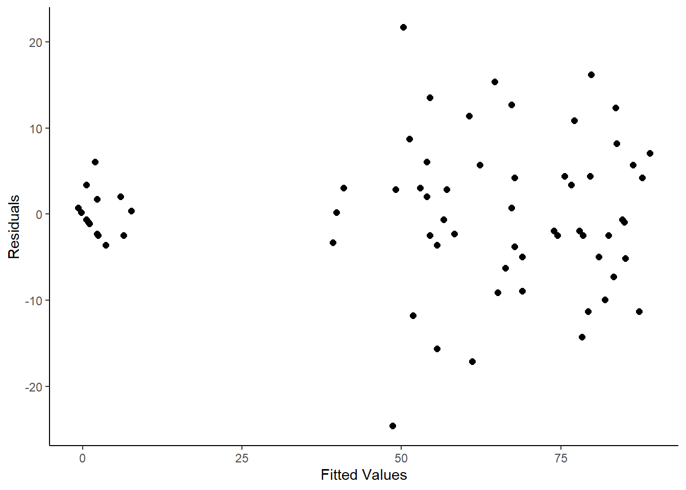
    RESFIT <-
           data.frame(
            residualvalue = residuals(fm4.2)
          , fittedvalue   = fitted.values(fm4.2)
          )

    ggplot(mapping = aes(
                          x = fitted.values(fm4.2)
                        , y = residuals(fm4.2))) +
    geom_point(size = 2) +
    labs(
        x = "Fitted Values"
      , y = "Residuals"
      ) +
      theme_classic()

Tip

Here the control pre-treatment was deleted.

 library(car)

 library(dae)

 library(dplyr)

 library(emmeans)

 library(ggplot2)

 library(lmerTest)

 library(magrittr)

 library(predictmeans)

 data(DataExam4.3)

 # Pg. 57
 fm4.4    <-
   aov(
       formula = percent ~ repl + treat*seedlot
     , data    = DataExam4.3 %>%
                  filter(treat != "control")
      )

  # Pg. 57
  anova(fm4.4)
Analysis of Variance Table

Response: percent
              Df Sum Sq Mean Sq F value      Pr(>F)    
repl           2   64.6   32.30  0.2511   0.7793606    
treat          2 5300.1 2650.07 20.6055 0.000001375 ***
seedlot        5 4148.1  829.63  6.4507   0.0002578 ***
treat:seedlot 10  961.2   96.12  0.7474   0.6759614    
Residuals     34 4372.7  128.61                        
---
Signif. codes:  0 '***' 0.001 '**' 0.01 '*' 0.05 '.' 0.1 ' ' 1

  model.tables(x = fm4.4, type = "means", se = TRUE)
Tables of means
Grand mean
         
67.85185 

 repl 
repl
    1     2     3 
69.11 66.44 68.00 

 treat 
treat
  nick   bw&s bw1min 
 56.89  65.78  80.89 

 seedlot 
seedlot
18211 18212 18217 18248 18249 18265 
77.33 69.33 63.11 53.33 64.89 79.11 

 treat:seedlot 
        seedlot
treat    18211 18212 18217 18248 18249 18265
  nick   65.33 54.67 57.33 40.00 49.33 74.67
  bw&s   78.67 68.00 54.67 52.00 61.33 80.00
  bw1min 88.00 85.33 77.33 68.00 84.00 82.67

Standard errors for differences of means
         repl treat seedlot treat:seedlot
        3.780 3.780   5.346         9.260
replic.    18    18       9             3

  emmeans(object = fm4.4, specs = ~ treat)
 treat  emmean   SE df lower.CL upper.CL
 nick     56.9 2.67 34     51.5     62.3
 bw&s     65.8 2.67 34     60.3     71.2
 bw1min   80.9 2.67 34     75.5     86.3

Results are averaged over the levels of: repl, seedlot 
Confidence level used: 0.95 

  emmeans(object = fm4.4, specs = ~ seedlot)
 seedlot emmean   SE df lower.CL upper.CL
 18211     77.3 3.78 34     69.7     85.0
 18212     69.3 3.78 34     61.7     77.0
 18217     63.1 3.78 34     55.4     70.8
 18248     53.3 3.78 34     45.7     61.0
 18249     64.9 3.78 34     57.2     72.6
 18265     79.1 3.78 34     71.4     86.8

Results are averaged over the levels of: repl, treat 
Confidence level used: 0.95 

  emmeans(object = fm4.4, specs = ~ treat * seedlot)
 treat  seedlot emmean   SE df lower.CL upper.CL
 nick   18211     65.3 6.55 34     52.0     78.6
 bw&s   18211     78.7 6.55 34     65.4     92.0
 bw1min 18211     88.0 6.55 34     74.7    101.3
 nick   18212     54.7 6.55 34     41.4     68.0
 bw&s   18212     68.0 6.55 34     54.7     81.3
 bw1min 18212     85.3 6.55 34     72.0     98.6
 nick   18217     57.3 6.55 34     44.0     70.6
 bw&s   18217     54.7 6.55 34     41.4     68.0
 bw1min 18217     77.3 6.55 34     64.0     90.6
 nick   18248     40.0 6.55 34     26.7     53.3
 bw&s   18248     52.0 6.55 34     38.7     65.3
 bw1min 18248     68.0 6.55 34     54.7     81.3
 nick   18249     49.3 6.55 34     36.0     62.6
 bw&s   18249     61.3 6.55 34     48.0     74.6
 bw1min 18249     84.0 6.55 34     70.7     97.3
 nick   18265     74.7 6.55 34     61.4     88.0
 bw&s   18265     80.0 6.55 34     66.7     93.3
 bw1min 18265     82.7 6.55 34     69.4     96.0

Results are averaged over the levels of: repl 
Confidence level used: 0.95 

4.2 Example 4.4 (Pg. 61)

Example 4.4 (Pg. 61)

An experiment supported by the Shell Company was planted at Toolara Forest Reserve near Gympie, Queensland, in February 1987 to study the effects of irrigation and fertiliser on four seedlots of Eucalyptus grandis. Because of the difficulty in applying the irrigation and fertiliser treatments individually to each 7 \(\times\) 6 plot of trees, the experiment was designed as a split-plot, with main-plot treatments, irrig and fert. There were two replicates of four main-plots each with four sub-plots.

 library(car)

 library(dae)

 library(dplyr)

 library(emmeans)

 library(ggplot2)

 library(lmerTest)

 library(magrittr)

 library(predictmeans)

 data(DataExam4.4)

 # Pg. 58
 fm4.6    <-
   aov(
       formula = height ~ repl + irrig*fert*seedlot +
                          Error(repl/irrig:fert)
     , data    = DataExam4.4
     )

 # Pg. 61
  summary(fm4.6)

Error: repl
     Df Sum Sq Mean Sq
repl  1 0.7564  0.7564

Error: repl:irrig:fert
           Df Sum Sq Mean Sq F value  Pr(>F)    
irrig       1    0.1     0.1   0.154   0.721    
fert        1  590.6   590.6 841.110 0.00009 ***
irrig:fert  1    0.0     0.0   0.010   0.926    
Residuals   3    2.1     0.7                    
---
Signif. codes:  0 '***' 0.001 '**' 0.01 '*' 0.05 '.' 0.1 ' ' 1

Error: Within
                   Df Sum Sq Mean Sq F value   Pr(>F)    
seedlot             3  39.65  13.218  19.680 0.000063 ***
irrig:seedlot       3   1.11   0.370   0.551   0.6572    
fert:seedlot        3   9.95   3.317   4.938   0.0185 *  
irrig:fert:seedlot  3   1.74   0.579   0.862   0.4874    
Residuals          12   8.06   0.672                     
---
Signif. codes:  0 '***' 0.001 '**' 0.01 '*' 0.05 '.' 0.1 ' ' 1

 # Pg. 61
 model.tables(x = fm4.6, type = "means")
Tables of means
Grand mean
         
10.00437 

 repl 
repl
     1      2 
10.158  9.851 

 irrig 
irrig
  none   plus 
 9.946 10.062 

 fert 
fert
  none   plus 
 5.708 14.301 

 seedlot 
seedlot
 Bulahdelah    Coffs SO Pomona pltn    Atherton 
     10.178      11.404      10.149       8.287 

 irrig:fert 
      fert
irrig  none   plus  
  none  5.635 14.257
  plus  5.781 14.344

 irrig:seedlot 
      seedlot
irrig  Bulahdelah Coffs SO Pomona pltn Atherton
  none 10.060     11.647   10.055       8.022  
  plus 10.295     11.160   10.242       8.552  

 fert:seedlot 
      seedlot
fert   Bulahdelah Coffs SO Pomona pltn Atherton
  none  5.687      6.790    5.410       4.945  
  plus 14.667     16.017   14.887      11.630  

 irrig:fert:seedlot 
, , seedlot = Bulahdelah

      fert
irrig  none   plus  
  none  5.275 14.845
  plus  6.100 14.490

, , seedlot = Coffs SO

      fert
irrig  none   plus  
  none  7.125 16.170
  plus  6.455 15.865

, , seedlot = Pomona pltn

      fert
irrig  none   plus  
  none  5.625 14.485
  plus  5.195 15.290

, , seedlot = Atherton

      fert
irrig  none   plus  
  none  4.515 11.530
  plus  5.375 11.730


 # Pg. 61
 emmeans(object = fm4.6, specs = ~ irrig)
 irrig emmean  SE  df asymp.LCL asymp.UCL
 none    9.95 NaN NaN       NaN       NaN
 plus   10.06 NaN NaN       NaN       NaN

Results are averaged over the levels of: repl, fert, seedlot 
Warning: EMMs are biased unless design is perfectly balanced 
Confidence level used: 0.95 

 emmip(object = fm4.6, formula  = ~ irrig) +
     theme_classic()