consensus of clusters

The criterion of the consensus is to produce many trees by means of boostrap and to such calculate the relative frequency with members of the clusters.

consensus(
  data,
  distance = c("binary", "euclidean", "maximum", "manhattan", "canberra", "minkowski",
    "gower", "chisq"),
  method = c("complete", "ward", "single", "average", "mcquitty", "median", "centroid"),
  nboot = 500,
  duplicate = TRUE,
  cex.text = 1,
  col.text = "red",
  ...
)

Arguments

data	data frame
distance	method distance, see dist()
method	method cluster, see hclust()
nboot	The number of bootstrap samples desired.
duplicate	control is TRUE other case is FALSE
cex.text	size text on percentage consensus
col.text	color text on percentage consensus
...	parameters of the plot dendrogram

Value

table.dend

The groups and consensus percentage

dendrogram

The class object is hclust, dendrogram plot

duplicate

Homonymous elements

Details

distance: "euclidean", "maximum", "manhattan", "canberra", "binary", "minkowski", "gower", "chisq". Method: "ward", "single", "complete", "average", "mcquitty", "median", "centroid". see functions: dist(), hclust() and daisy() of cluster.

References

An Introduction to the Boostrap. Bradley Efron and Robert J. Tibshirani. 1993. Chapman and Hall/CRC

See also

hclust, hgroups, hcut

Examples

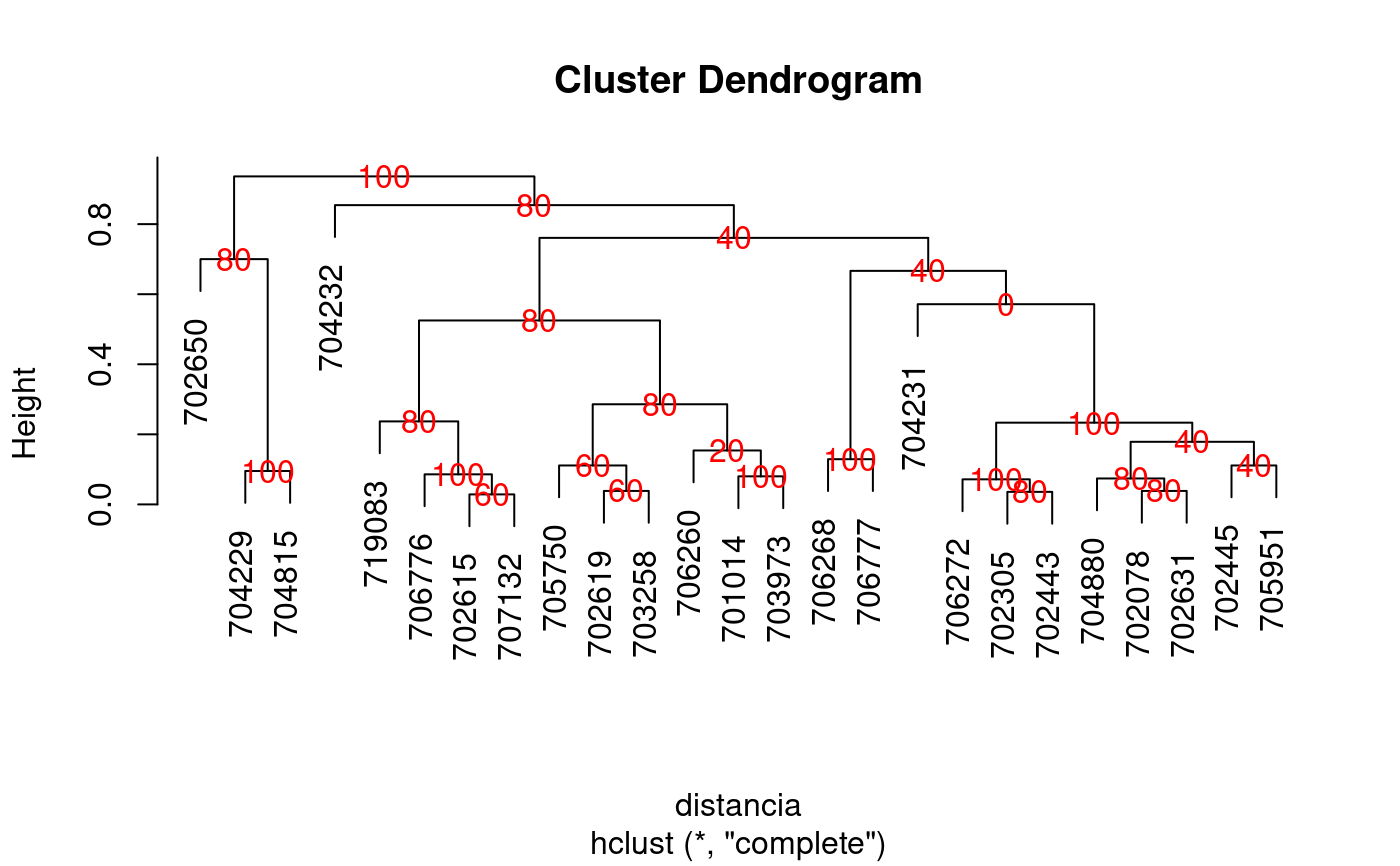
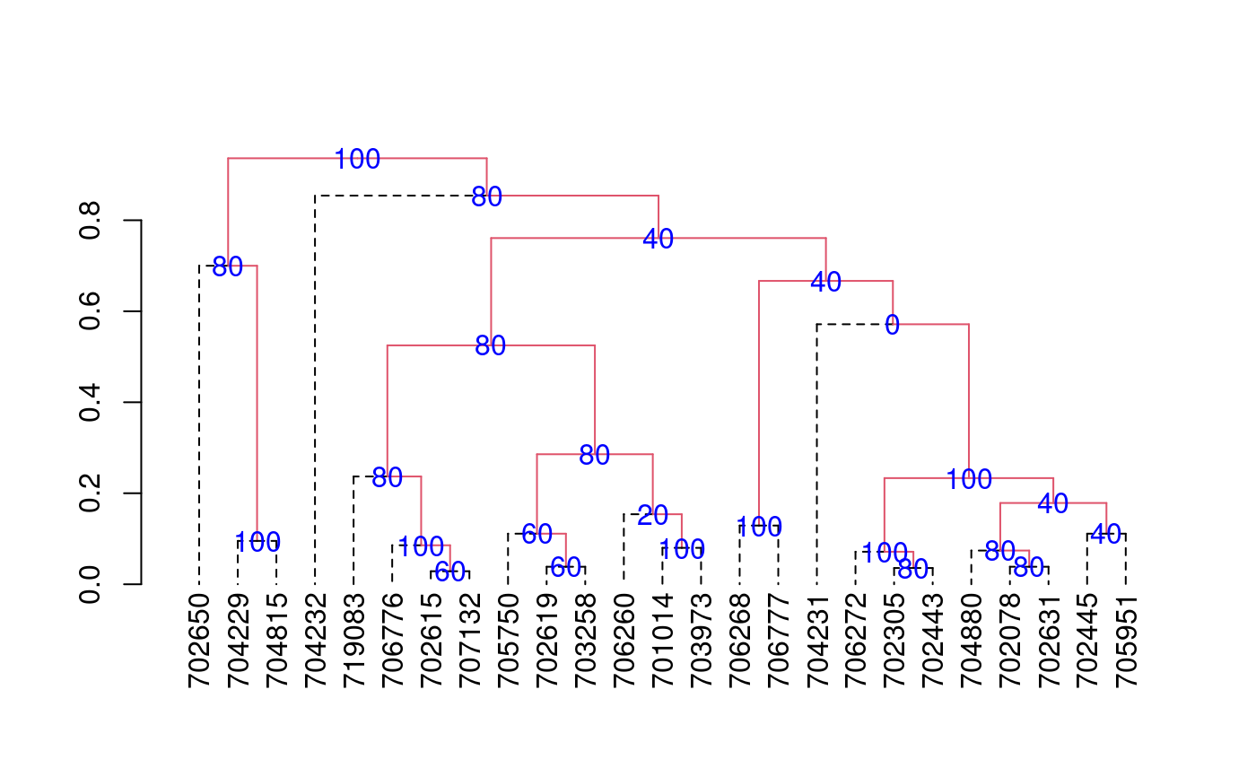
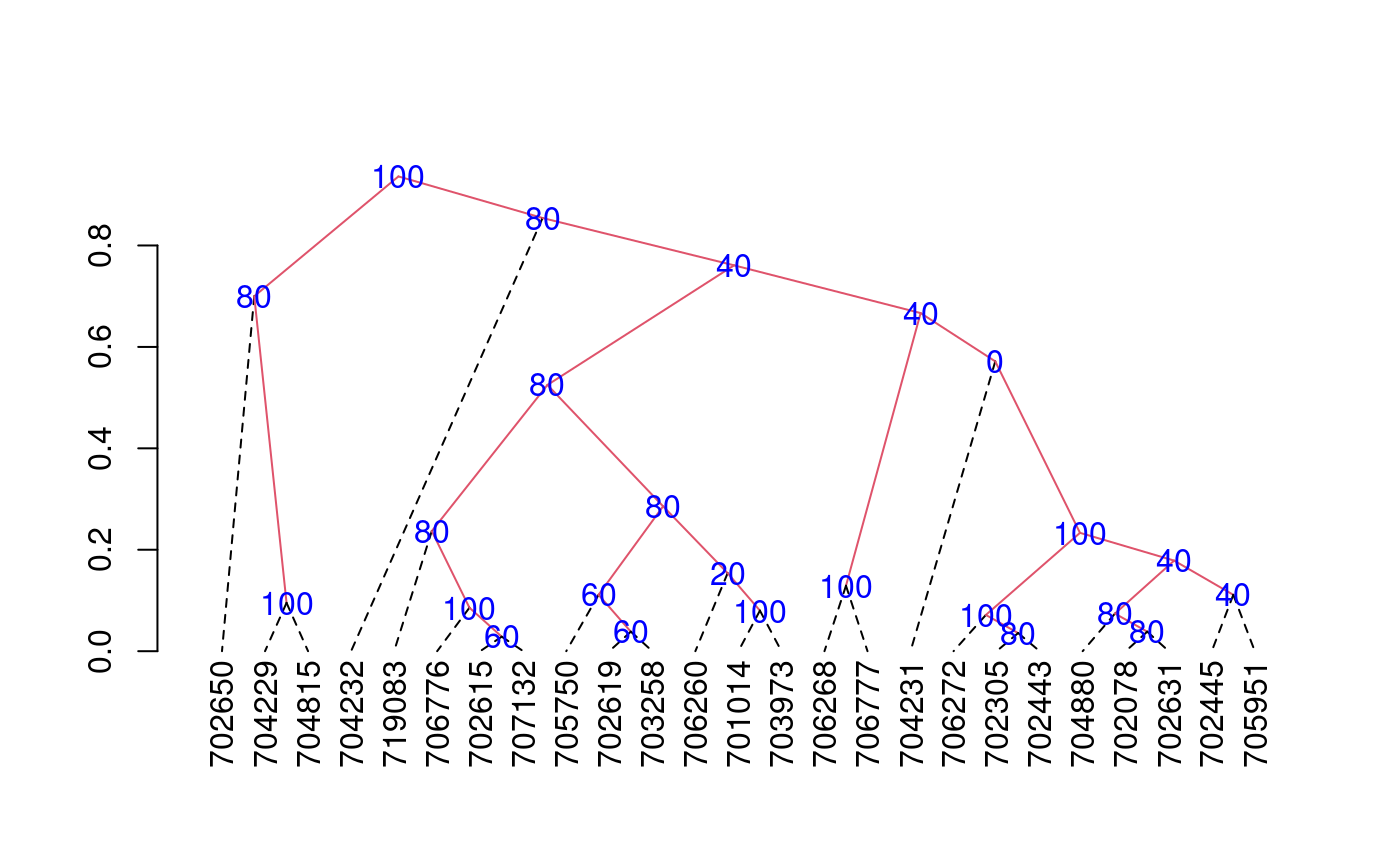
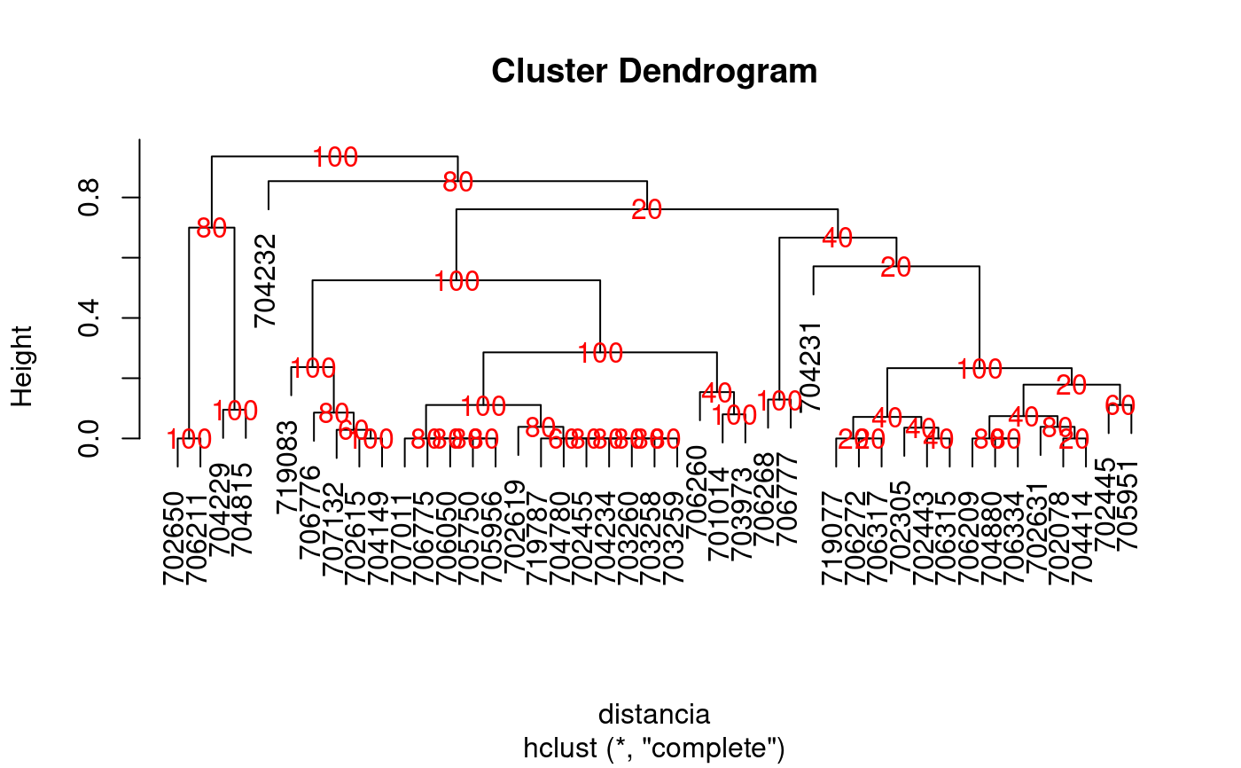
library(agricolae)
data(pamCIP)
# only code
rownames(pamCIP)<-substr(rownames(pamCIP),1,6)
output<-consensus( pamCIP,distance="binary", method="complete",nboot=5)
#> 
#> Duplicates: 18
#> New data  : 25 Records
#> 
#> Consensus hclust
#> 
#> Method distance: binary
#> Method cluster : complete
#> rows and cols  : 25 107
#> n-bootstrap    : 5
#> Run time       : 0.6697083 secs 
#> 
# Order consensus
Groups<-output$table.dend[,c(6,5)]
Groups<-Groups[order(Groups[,2],decreasing=TRUE),]
print(Groups)
#>                                                               groups percentage
#> 5                                                             3-4-21        100
#> 7                                                               1-11        100
#> 8                                                            6-22-24        100
#> 9                                                              12-15        100
#> 12                                                             20-23        100
#> 15                                                2-3-4-5-8-16-18-21        100
#> 24 1-2-3-4-5-6-7-8-9-10-11-12-13-14-15-16-17-18-19-20-21-22-23-24-25        100
#> 2                                                                3-4         80
#> 3                                                                2-8         80
#> 6                                                             2-8-16         80
#> 16                                                        6-22-24-25         80
#> 17                                                   1-7-10-11-17-19         80
#> 18                                        1-6-7-10-11-17-19-22-24-25         80
#> 21                                                           9-12-15         80
#> 23         1-2-3-4-5-6-7-8-10-11-13-14-16-17-18-19-20-21-22-23-24-25         80
#> 1                                                               6-24         60
#> 4                                                               7-10         60
#> 11                                                           7-10-17         60
#> 10                                                              5-18         40
#> 14                                                       2-5-8-16-18         40
#> 20                                       2-3-4-5-8-13-16-18-20-21-23         40
#> 22            1-2-3-4-5-6-7-8-10-11-13-16-17-18-19-20-21-22-23-24-25         40
#> 13                                                           1-11-19         20
#> 19                                             2-3-4-5-8-13-16-18-21          0
## Identification of the codes with the numbers.
cbind(output$dendrogram$labels)
#>       [,1]    
#>  [1,] "701014"
#>  [2,] "702078"
#>  [3,] "702305"
#>  [4,] "702443"
#>  [5,] "702445"
#>  [6,] "702615"
#>  [7,] "702619"
#>  [8,] "702631"
#>  [9,] "702650"
#> [10,] "703258"
#> [11,] "703973"
#> [12,] "704229"
#> [13,] "704231"
#> [14,] "704232"
#> [15,] "704815"
#> [16,] "704880"
#> [17,] "705750"
#> [18,] "705951"
#> [19,] "706260"
#> [20,] "706268"
#> [21,] "706272"
#> [22,] "706776"
#> [23,] "706777"
#> [24,] "707132"
#> [25,] "719083"
## To reproduce dendrogram
dend<-output$dendrogram
data<-output$table.dend
plot(dend)
text(data[,3],data[,4],data[,5])
# Other examples
# classical dendrogram
dend<-as.dendrogram(output$dendrogram)
plot(dend,type="r",edgePar = list(lty=1:2, col=2:1))
text(data[,3],data[,4],data[,5],col="blue",cex=1)
plot(dend,type="t",edgePar = list(lty=1:2, col=2:1))
text(data[,3],data[,4],data[,5],col="blue",cex=1)
## Without the control of duplicates
output<-consensus( pamCIP,duplicate=FALSE,nboot=5)
#> 
#> Consensus hclust
#> 
#> Method distance: binary
#> Method cluster : complete
#> rows and cols  : 43 107
#> n-bootstrap    : 5
#> Run time       : 0.03551149 secs 
#> 
## using distance gower, require cluster package.
# output<-consensus( pamCIP,distance="gower", method="complete",nboot=5)