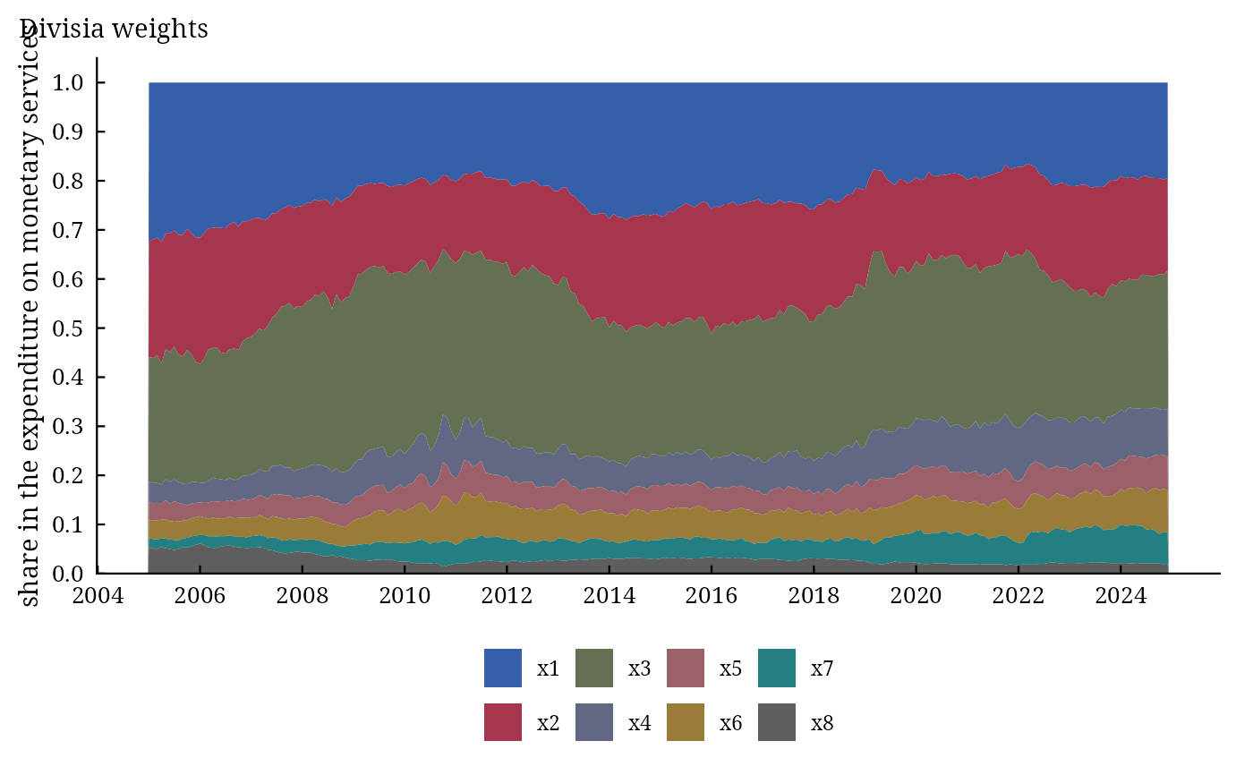
dmai_user_cost() gives, for every date and component, the rate, the user cost
\(\pi_{it} = (R_t - r_{it})/(1 + R_t)\) (Barnett 1978) and the share of the
component in the expenditure on monetary services, the weights of the Divisia index.
Usage
dmai_user_cost(
  .data,
  date = "Date",
  x = NULL,
  r = NULL,
  benchmark = NULL,
  percent = TRUE
)

# Default S3 method
dmai_user_cost(
  .data,
  date = "Date",
  x = NULL,
  r = NULL,
  benchmark = NULL,
  percent = TRUE
)
Arguments
- .data
a data frame with one row per date: a date column and, for every component, a quantity column and a rate column (named
x1,x2, ... andr1,r2, ... unlessxandrare given).- date
name of the date column (default
"Date").- x
names of the quantity columns (default
NULL:x1,x2, ...).- r
names of the rate columns, in the order of
x(defaultNULL:r1,r2, ...).- benchmark
the benchmark rate:
NULL(default, the largest component rate), a column name, a number or one value per row of.data, in the units of the rates.- percent
logical; are the rates in percent (default
TRUE) or decimal?
Value
An object of class c("dmai_user_cost", "dmai_result", "list"): components (date,
component, quantity, rate, user cost, share), benchmark (the benchmark rate and whether the upper
envelope raised it) and settings. plot() draws the shares over time.
References
Barnett, W. A. (1978). The user cost of money. Economics Letters, 1(2), 145–149. doi:10.1016/0165-1765(78)90051-4
See also
Other dmai analyses:
dmai(),
dmai_compare(),
dmai_moments()
Author
Muhammad Yaseen (myaseen208@gmail.com)
Examples
data(money_sim)
uc <-
  dmai_user_cost(
      .data     = money_sim
    , date      = "Date"
    , x         = NULL
    , r         = NULL
    , benchmark = "rb"
    , percent   = TRUE
    )
uc
#> User costs of 8 components, 240 dates
#> =====================================
#> Averages over the dates:
#>    component mean_rate mean_user_cost mean_share last_share
#>       <fctr>     <num>          <num>      <num>      <num>
#> 1:        x1     0.000        0.08124    0.22914    0.19497
#> 2:        x2     0.000        0.08124    0.20366    0.18827
#> 3:        x3     3.050        0.05360    0.30779    0.28085
#> 4:        x4     4.903        0.03662    0.07486    0.09851
#> 5:        x5     5.414        0.03193    0.05076    0.06799
#> 6:        x6     5.921        0.02727    0.06106    0.08527
#> 7:        x7     6.647        0.02059    0.04325    0.06416
#> 8:        x8     1.316        0.06916    0.02949    0.01998
#>
#> Sources: Barnett (1978). Full references: dmai_cite(x).
plot(x = uc)