Regression Analysis with Python

Python

Statistics

Regression Analysis

Regression Analysis with Python.

Author

Affiliation

Muhammad Yaseen

Dept of Math & Stat, Univ of Agriculture, Faisalabad Pakistan

Published

September 20, 2018

Introduction

In God we trust, all others must bring data. (W. Edwards Deming)

In Data we trust, all others must bring data.

Statistics

Statistics is the science of uncertainty & variability

Statistics turns data into information

Data -> Information -> Knowledge -> Wisdom

Data Driven Decisions (3Ds)

Statistics is the interpretation of Science

Statistics is the Art & Science of learning from data

Variable

Characteristic that may vary from individual to individual

Height, Weight, CGPA etc

Measurement

Process of assigning numbers or labels to objects or states in accordance with logically accepted rules

Measurement Scales

Nominal Scale: Obersvations may be classified into mutually exclusive & exhaustive classes or categories

Ordinal Scale: Obersvations may be ranked

Interval Scale: Difference between obersvations is meaningful

Ratio Scale: Ratio between obersvations is meaningful & true zero point

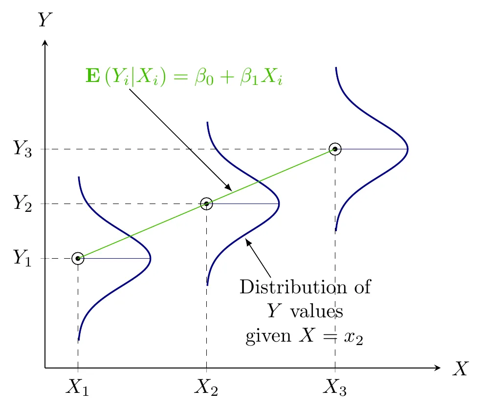
Regression Analysis

Quantifying dependency of a normal response on quantitative explanatory variable(s)

Simple Linear Regression

Quantifying dependency of a normal response on a quantitative explanatory variable

Example

Weekly Income ($)	Weekly Expenditures ($)
80	70
100	65
120	90
140	95
160	110
180	115
200	120
220	140
240	155
260	150

Income = [80, 100, 120, 140, 160, 180, 200, 220, 240, 260]
Expend = [70, 65, 90, 95, 110, 115, 120, 140, 155, 150]

import pandas as pd
df1 = pd.DataFrame(
 {
   "Income": Income
 , "Expend": Expend
 }
 )

print(df1)

   Income  Expend
0      80      70
1     100      65
2     120      90
3     140      95
4     160     110
5     180     115
6     200     120
7     220     140
8     240     155
9     260     150

from matplotlib import pyplot as plt
fig = plt.figure()
plt.scatter(
  df1["Income"]
, df1["Expend"]
, color = "green"
, marker = "o"
)
plt.title("Scatter plot of Weekly Income (\$) and Weekly Expenditures (\$)")
plt.xlabel("Weekly Income (\$)")
plt.ylabel("Weekly Expenditures (\$)")
plt.show()

from statsmodels.formula.api import ols
from statsmodels.stats.anova import anova_lm
Reg1 = ols(formula = "Expend ~ Income", data = df1)
Fit1 = Reg1.fit()
print(Fit1.summary())

                            OLS Regression Results                            
==============================================================================
Dep. Variable:                 Expend   R-squared:                       0.962
Model:                            OLS   Adj. R-squared:                  0.957
Method:                 Least Squares   F-statistic:                     202.9
Date:                Sat, 12 Apr 2025   Prob (F-statistic):           5.75e-07
Time:                        20:11:21   Log-Likelihood:                -31.781
No. Observations:                  10   AIC:                             67.56
Df Residuals:                       8   BIC:                             68.17
Df Model:                           1                                         
Covariance Type:            nonrobust                                         
==============================================================================
                 coef    std err          t      P>|t|      [0.025      0.975]
------------------------------------------------------------------------------
Intercept     24.4545      6.414      3.813      0.005       9.664      39.245
Income         0.5091      0.036     14.243      0.000       0.427       0.592
==============================================================================
Omnibus:                        1.060   Durbin-Watson:                   2.680
Prob(Omnibus):                  0.589   Jarque-Bera (JB):                0.777
Skew:                          -0.398   Prob(JB):                        0.678
Kurtosis:                       1.891   Cond. No.                         561.
==============================================================================

Notes:
[1] Standard Errors assume that the covariance matrix of the errors is correctly specified.

print(Fit1.params)

Intercept    24.454545
Income        0.509091
dtype: float64

print(Fit1.fittedvalues)

0     65.181818
1     75.363636
2     85.545455
3     95.727273
4    105.909091
5    116.090909
6    126.272727
7    136.454545
8    146.636364
9    156.818182
dtype: float64

print(Fit1.resid)

0     4.818182
1   -10.363636
2     4.454545
3    -0.727273
4     4.090909
5    -1.090909
6    -6.272727
7     3.545455
8     8.363636
9    -6.818182
dtype: float64

print(Fit1.bse)

Intercept    6.413817
Income       0.035743
dtype: float64

print(Fit1.centered_tss)

8890.0

print(anova_lm(Fit1))

           df       sum_sq      mean_sq           F        PR(>F)
Income    1.0  8552.727273  8552.727273  202.867925  5.752746e-07
Residual  8.0   337.272727    42.159091         NaN           NaN

fig = plt.figure()
plt.scatter(
  df1["Income"]
, df1["Expend"]
, color = "green"
, marker = "o"
)
plt.plot(df1["Income"], Fit1.fittedvalues)
plt.title("Regression plot of Weekly Income (\$) and Weekly Expenditures (\$)")
plt.xlabel("Weekly Income (\$)")
plt.ylabel("Weekly Expenditures (\$)")
plt.show()

Multiple Linear Regression

Quantifying dependency of a normal response on two or more quantitative explanatory variables

Example

Fertilizer (Kg)	Rainfall (mm)	Yield (Kg)
100	10	40
200	20	50
300	10	50
400	30	70
500	20	65
600	20	65
700	30	80

import numpy as np
Fertilizer = np.arange(100, 800, 100)
Rainfall   = [10, 20, 10, 30, 20, 20, 30]
Yield      = [40, 50, 50, 70, 65, 65, 80]

import pandas as pd
df2 = pd.DataFrame(
 {
   "Fertilizer": Fertilizer
 , "Rainfall": Rainfall
 , "Yield": Yield
 }
 )

print(df2)

   Fertilizer  Rainfall  Yield
0         100        10     40
1         200        20     50
2         300        10     50
3         400        30     70
4         500        20     65
5         600        20     65
6         700        30     80

from mpl_toolkits.mplot3d import Axes3D
from matplotlib import pyplot as plt
fig = plt.figure()
ax = fig.add_subplot(111, projection = "3d")
ax.scatter(
  df2["Fertilizer"]
, df2["Rainfall"]
, df2["Yield"]
, color = "green"
, marker = "o"
, alpha  = 1
)
ax.set_xlabel("Fertilizer")
ax.set_ylabel("Rainfall")
ax.set_zlabel("Yield")
plt.show()

from statsmodels.formula.api import ols
from statsmodels.stats.anova import anova_lm
Reg2 = ols(formula = "Yield ~ Fertilizer + Rainfall", data = df2)
Fit2 = Reg2.fit()
print(Fit2.summary())

                            OLS Regression Results                            
==============================================================================
Dep. Variable:                  Yield   R-squared:                       0.981
Model:                            OLS   Adj. R-squared:                  0.972
Method:                 Least Squares   F-statistic:                     105.3
Date:                Sat, 12 Apr 2025   Prob (F-statistic):           0.000347
Time:                        20:11:23   Log-Likelihood:                -13.848
No. Observations:                   7   AIC:                             33.70
Df Residuals:                       4   BIC:                             33.53
Df Model:                           2                                         
Covariance Type:            nonrobust                                         
==============================================================================
                 coef    std err          t      P>|t|      [0.025      0.975]
------------------------------------------------------------------------------
Intercept     28.0952      2.491     11.277      0.000      21.178      35.013
Fertilizer     0.0381      0.006      6.532      0.003       0.022       0.054
Rainfall       0.8333      0.154      5.401      0.006       0.405       1.262
==============================================================================
Omnibus:                          nan   Durbin-Watson:                   2.249
Prob(Omnibus):                    nan   Jarque-Bera (JB):                0.705
Skew:                          -0.408   Prob(JB):                        0.703
Kurtosis:                       1.677   Cond. No.                     1.28e+03
==============================================================================

Notes:
[1] Standard Errors assume that the covariance matrix of the errors is correctly specified.
[2] The condition number is large, 1.28e+03. This might indicate that there are
strong multicollinearity or other numerical problems.

print(Fit2.params)

Intercept     28.095238
Fertilizer     0.038095
Rainfall       0.833333
dtype: float64

print(Fit2.fittedvalues)

0    40.238095
1    52.380952
2    47.857143
3    68.333333
4    63.809524
5    67.619048
6    79.761905
dtype: float64

print(Fit2.resid)

0   -0.238095
1   -2.380952
2    2.142857
3    1.666667
4    1.190476
5   -2.619048
6    0.238095
dtype: float64

print(Fit2.bse)

Intercept     2.491482
Fertilizer    0.005832
Rainfall      0.154303
dtype: float64

print(Fit2.centered_tss)

1150.0

print(anova_lm(Fit2))

             df      sum_sq     mean_sq           F    PR(>F)
Fertilizer  1.0  972.321429  972.321429  181.500000  0.000176
Rainfall    1.0  156.250000  156.250000   29.166667  0.005690
Residual    4.0   21.428571    5.357143         NaN       NaN

from mpl_toolkits.mplot3d import Axes3D
from matplotlib import pyplot as plt
import numpy as np
import pandas as pd
from matplotlib import cm

fig = plt.figure()
ax = fig.add_subplot(111, projection="3d")

ax.scatter(
    df2["Fertilizer"],
    df2["Rainfall"],
    df2["Yield"],
    color="green",
    marker="o",
    alpha=1
)

ax.set_xlabel("Fertilizer")
ax.set_ylabel("Rainfall")
ax.set_zlabel("Yield")

x_surf = np.arange(100, 720, 20)
y_surf = np.arange(10, 32, 2)
x_surf, y_surf = np.meshgrid(x_surf, y_surf)

exog = pd.DataFrame({
    "Fertilizer": x_surf.ravel(),
    "Rainfall": y_surf.ravel()
})

out = Fit2.predict(exog=exog)

# ✅ Convert to numpy before reshaping
z_surf = out.to_numpy().reshape(x_surf.shape)

ax.plot_surface(
    x_surf,
    y_surf,
    z_surf,
    rstride=1,
    cstride=1,
    color="None",
    alpha=0.4
)

plt.show()

Polynomial Regression Analysis

Quantifying non-linear dependency of a normal response on quantitative explanatory variable(s)

Example

An experiment was conducted to evaluate the effects of different levels of nitrogen. Three levels of nitrogen: 0, 10 and 20 grams per plot were used in the experiment. Each treatment was replicated twice and data is given below:

Nitrogen	Yield
0	5
0	7
10	15
10	17
20	9
20	11

Nitrogen = [0, 0, 10, 10, 20, 20]
Yield    = [5, 7, 15, 17,  9, 11]

import pandas as pd
df3 = pd.DataFrame(
 {
   "Nitrogen": Nitrogen
 , "Yield": Yield
 }
 )

print(df3)

   Nitrogen  Yield
0         0      5
1         0      7
2        10     15
3        10     17
4        20      9
5        20     11

from matplotlib import pyplot as plt
fig = plt.figure()
plt.scatter(
  df3["Nitrogen"]
, df3["Yield"]
, color = "green"
, marker = "o"
)
plt.title("Scatter plot of Nitrogen and Yield")
plt.xlabel("Nitrogen")
plt.ylabel("Yield")
plt.show()

from statsmodels.formula.api import ols
from statsmodels.stats.anova import anova_lm
Reg3 = ols(formula = "Yield ~ Nitrogen + I(Nitrogen**2)", data = df3)
Fit3 = Reg3.fit()
print(Fit3.summary())

                            OLS Regression Results                            
==============================================================================
Dep. Variable:                  Yield   R-squared:                       0.944
Model:                            OLS   Adj. R-squared:                  0.907
Method:                 Least Squares   F-statistic:                     25.33
Date:                Sat, 12 Apr 2025   Prob (F-statistic):             0.0132
Time:                        20:11:25   Log-Likelihood:                -8.5136
No. Observations:                   6   AIC:                             23.03
Df Residuals:                       3   BIC:                             22.40
Df Model:                           2                                         
Covariance Type:            nonrobust                                         
====================================================================================
                       coef    std err          t      P>|t|      [0.025      0.975]
------------------------------------------------------------------------------------
Intercept            6.0000      1.000      6.000      0.009       2.818       9.182
Nitrogen             1.8000      0.255      7.060      0.006       0.989       2.611
I(Nitrogen ** 2)    -0.0800      0.012     -6.532      0.007      -0.119      -0.041
==============================================================================
Omnibus:                          nan   Durbin-Watson:                   3.333
Prob(Omnibus):                    nan   Jarque-Bera (JB):                1.000
Skew:                           0.000   Prob(JB):                        0.607
Kurtosis:                       1.000   Cond. No.                         418.
==============================================================================

Notes:
[1] Standard Errors assume that the covariance matrix of the errors is correctly specified.

print(Fit3.params)

Intercept           6.00
Nitrogen            1.80
I(Nitrogen ** 2)   -0.08
dtype: float64

print(Fit3.fittedvalues)

0     6.0
1     6.0
2    16.0
3    16.0
4    10.0
5    10.0
dtype: float64

print(Fit3.resid)

0   -1.0
1    1.0
2   -1.0
3    1.0
4   -1.0
5    1.0
dtype: float64

print(Fit3.bse)

Intercept           1.000000
Nitrogen            0.254951
I(Nitrogen ** 2)    0.012247
dtype: float64

print(Fit3.centered_tss)

107.33333333333334

print(anova_lm(Fit3))

                   df     sum_sq    mean_sq          F    PR(>F)
Nitrogen          1.0  16.000000  16.000000   8.000000  0.066276
I(Nitrogen ** 2)  1.0  85.333333  85.333333  42.666667  0.007292
Residual          3.0   6.000000   2.000000        NaN       NaN

fig = plt.figure()
plt.scatter(
  df3["Nitrogen"]
, df3["Yield"]
, color = "green"
, marker = "o"
)
plt.plot(df3["Nitrogen"], Fit3.fittedvalues)
plt.title("Regression plot of Nitrogen and Yield")
plt.xlabel("Nitrogen")
plt.ylabel("Yield")
plt.show()

Citation

BibTeX citation:

@online{ryan2018,
  author = {Ryan, Jadey and Yaseen, Muhammad},
  title = {Regression {Analysis} with {Python}},
  date = {2018-09-20},
  url = {https://myaseen208.com/blog/2018-09-20_RegPython/2018-09-20_RegPython.html},
  langid = {en}
}

For attribution, please cite this work as:

Ryan, Jadey, and Muhammad Yaseen. 2018. “Regression Analysis with Python.” September 20, 2018. https://myaseen208.com/blog/2018-09-20_RegPython/2018-09-20_RegPython.html.

Introduction

Statistics

Variable

Measurement

Measurement Scales

Regression Analysis

Simple Linear Regression

Example

Multiple Linear Regression

Example

Polynomial Regression Analysis

Example

Citation

Subscribe to get notified about new content.