Random generation by Montecarlo

Random generation form data, use function density and parameters

montecarlo(data, k, ...)

Arguments

data	vector or object(hist, graph.freq)
k	number of simulations
...	Other parameters of the function density, only if data is vector

Value

Generate random numbers with empirical distribution.

See also

density

Examples

library(agricolae)
r<-rnorm(50, 10,2)
montecarlo(r, k=100, kernel="epanechnikov")
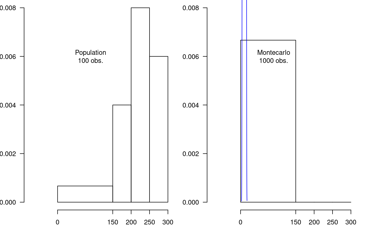
#>   [1] 13.051613  8.468413  9.827569 13.304479  9.922394 15.959574 12.166581
#>   [8]  4.232905  8.879321  8.310372 10.017219  9.068971  7.551774 12.672313
#>  [15]  7.867856 13.936644 12.545880  4.359338  9.448270  7.172474  3.790389
#>  [22] 12.261406  9.258620  9.954002  7.077649 12.356231 12.703922 12.293014
#>  [29] 13.020004  8.784496  6.255834 10.522951 12.387839 11.755674  7.330516
#>  [36] 10.048827 15.485450  7.362124 10.586168 10.017219 14.094686 12.198189
#>  [43] 11.376374 14.063077  8.436805  9.416662  8.373589 12.798747 14.537201
#>  [50] 10.270085  6.982825  8.942537  8.974146  6.856392 13.272871  9.574703
#>  [57] 11.376374  6.224226 11.724065 14.568810 11.123508  8.594846  8.594846
#>  [64]  4.422555  8.752888  6.635134 10.270085  9.479878 12.356231 10.270085
#>  [71]  7.046041  7.994289  8.658063 11.629240 14.410768 11.882107  4.991504
#>  [78]  8.468413  7.362124 10.522951  9.195404 12.767138  7.867856 11.976931
#>  [85] 14.284335 12.261406  8.089114 12.925180  8.120722 11.060292  9.637919
#>  [92] 12.640705 14.252727  8.057506 10.712601 11.724065 10.522951  9.416662
#>  [99] 12.451056  7.456949
# other example
h<-hist(r,plot=FALSE)
montecarlo(h, k=100)
#>   [1]  8.890895  8.176087 15.853777 13.364009  8.263260  9.892125 11.271305
#>   [8]  9.137233 15.504633  7.047226  8.177902 10.937915  9.897187  9.228510
#>  [15] 12.536734  7.281644  6.045639 11.181868 11.712868  9.792405  8.586787
#>  [22]  9.058353  9.915716 10.601531 11.954634  6.321239 10.213165 12.270448
#>  [29] 10.085454 10.729684  8.551028  9.506762 15.778672 11.753025  9.717662
#>  [36]  6.835867  8.349339  4.439961  9.153647  6.896786  8.756314  7.783035
#>  [43] 13.586012 15.260068  9.506302 10.413303 10.913267 11.507782  8.235493
#>  [50]  6.718644  9.556069  7.040178 12.759613 10.886160 10.015279 11.369920
#>  [57]  6.897374  9.502858 14.905502  6.883863  6.519658  6.932246 11.320026
#>  [64] 14.811630  6.419458  9.763918 11.640892  9.108587 11.968482  8.509126
#>  [71]  7.181207  6.639744  7.465228 10.855295  9.453499  8.872006  8.982241
#>  [78] 13.185733  7.876673 12.035770  8.357959 10.666061 12.933377  6.811592
#>  [85]  9.487861 10.462159  9.641544 11.810421  6.204041  8.833070  7.538797
#>  [92] 15.589634 10.831597 11.909540 10.709788 12.640547 12.711105 10.615331
#>  [99] 13.987957 11.605399
# other example
breaks<-c(0, 150, 200, 250, 300)
counts<-c(10, 20, 40, 30)
par(mfrow=c(1,2),cex=0.8,mar=c(2,3,0,0))
h1<-graph.freq(x=breaks,counts=counts,plot=FALSE)
r<-montecarlo(h, k=1000)
plot(h1,frequency = 3,ylim=c(0,0.008))
text(90,0.006,"Population\n100 obs.")
h2<-graph.freq(r,breaks,frequency = 3,ylim=c(0,0.008))
lines(density(r),col="blue")
text(90,0.006,"Montecarlo\n1000 obs.")