[1] 0.6065307[1] 0.2386512
After careful study of this chapter, you should be able to do the following:
Experiment
Random
Random experiment
Figure 3.1 illustrates the relationship between a mathematical model and the physical system it represents. While models like Newton’s laws are not perfect abstractions, they are useful for analyzing and approximating system performance. Once validated with measurements, models can help understand, describe, and predict a system’s response to inputs.
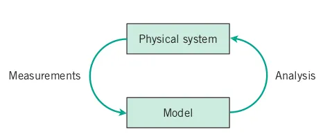
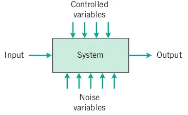
Figure 3.2 illustrates a model where uncontrollable variables (noise) interact with controllable variables to produce system outputs. Due to the noise, identical controllable settings yield varying outputs upon measurement.
For measuring current in a copper wire, Ohm’s law may suffice as a model. However, if variations are significant, the model may need to account for them (see Figure 3.3).

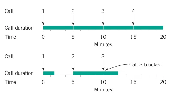
In designing a voice communication system, a model is required for call frequency and duration. Even if calls occur and last precisely 5 minutes on average, variations in timing or duration can lead to call blocking, necessitating multiple lines (see Figure 3.4).
A random variable is a numerical variable whose measured value can change from one replicate of the experiment to another.
Used to quantify likelihood or chance
Used to represent risk or uncertainty in engineering applications
Can be interpreted as our degree of belief or relative frequency
Probability statements describe the likelihood that particular values occur.
The likelihood is quantified by assigning a number from the interval [0, 1] to the set of values (or a percentage from 0 to 100%).
Higher numbers indicate that the set of values is more likely.
A probability is usually expressed in terms of a random variable.
For the part length example, X denotes the part length and the probability statement can be written in either of the following forms P\left(X\in\left[10.8,11.2\right]\right)=0.25 or P\left(10.8\leq X\leq11.2\right)=0.25.
Both equations state that the probability that the random variable X assumes a value in \left[10.8,11.2\right] is 0.25.
Given a set E, the complement of E is the set of elements that are not in E. The complement is denoted as E^{\prime} or E^{c}.
The sets E_{1}, E_{2} ,\ldots,E_{k} are mutually exclusive if the intersection of any pair is empty. That is, each element is in one and only one of the sets E_{1}, E_{2} ,\ldots,E_{k}.
The probability distribution or simply distribution of a random variable X is a description of the set of the probabilities associated with the possible values for X.
The probability density function (or pdf) f(x) of a continuous random variable X is used to determine probabilities as follows: P(a < X < b) = \int_{a}^{b} f(x)\,dx
The properties of the pdf are
If X is a continuous random variable, for any x1 and x2, P\left(x_{1}\leq X\leq x_{2}\right)=P\left(x_{1}<X\leq x_{2}\right)=P\left(x_{1}\leq X<x_{2}\right)=P\left(x_{1}<X<x_{2}\right)
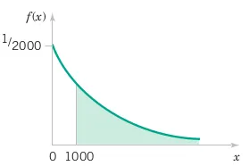
Let the continuous random variable X denote the distance in micrometers from the start of a track on a magnetic disk until the first flaw. Historical data show that the distribution of X can be modeled by the probability density function (pdf):
f(x) = \frac{1}{2000} e^{-x/2000}, \quad x \geq 0.
For what proportion of disks is the distance to the first flaw greater than 1000 micrometers? What proportion of parts is between 1000 and 2000 micrometers?
The probability that the distance to the first flaw is greater than 1000 micrometers is given by:
\begin{align*} P(X > 1000) &= \int_{1000}^{\infty} f(x)\,dx \\ &= \int_{1000}^{\infty} \frac{1}{2000} e^{-x/2000} \,dx. \end{align*}
To evaluate the integral, we use the formula for the integral of an exponential function:
\int e^{-ax} \,dx = \frac{e^{-ax}}{-a}.
Here, a = \frac{1}{2000}, so:
\begin{align*} P(X > 1000) &= \left[ -e^{-x/2000} \right]_{1000}^{\infty} \\ &= \left( 0 - \left( -e^{-1000/2000} \right) \right) \\ &= e^{-1/2} \\ &\approx 0.6065. \end{align*}
Thus, the proportion of disks where the distance to the first flaw is greater than 1000 micrometers is approximately 0.6065.
The probability that the distance to the first flaw is between 1000 and 2000 micrometers is given by:
\begin{align*} P(1000 \leq X \leq 2000) &= \int_{1000}^{2000} f(x)\,dx \\ &= \int_{1000}^{2000} \frac{1}{2000} e^{-x/2000} \,dx. \\ & = \left[ -e^{-x/2000} \right]_{1000}^{2000} \\ &= e^{-1/2} - e^{-1}\\ &= 0.6065 - 0.3679 \\ &= 0.2386. \end{align*}
Therefore, the proportion of parts with a flaw distance between 1000 and 2000 micrometers is approximately 0.2386.
[1] 0.6065307[1] 0.2386512pdf1 <- function(x) {(1/2000) * exp(-x/2000)}
integrate(
f = pdf1
, lower = 1000
, upper = Inf
)$value
integrate(
f = pdf1
, lower = 1000
, upper = 2000
)$valueThe cumulative distribution function (or cdf) of a continuous random variable X with probability density function f(x) is F(X) = P(X \leq x) = \int_{-\infty}^{x} f(u)\,du for -\infty < x < \infty.
For a continuous random variable X, the definition can also be F(x)= P(X < x) because P(X = x) = 0.
The cumulative distribution function F(x) can be related to the probability density function f(x) and can be used to obtain probabilities as follows.
\begin{align*} P(a<X<b) & = \int_{a}^{b} f(x)\,dx \\ & = \int_{-\infty}^{b} f(x)\,dx - \int_{-\infty}^{a} f(x)\,dx \\ & = F(b) - F(a) \end{align*} Furthermore, the graph of a cdf has specific properties. Because F(x) provides probabilities, it is always nonnegative. Furthermore, as x increases, F(x) is nondecreasing. Finally, as x tends to infinity, F (x) = P(X \leq x) tends to 1.
Let the continuous random variable X denote the distance in micrometers from the start of a track on a magnetic disk until the first flaw. Historical data show that the distribution of X can be modeled by the probability density function (pdf):
f(x) = \frac{1}{2000} e^{-x/2000}, \quad x \geq 0.
The cdf is determined from
\begin{align*} F(X) & = P(X \leq x) = \int_{0}^{x} \frac{1}{2000} e^{-u/2000}\,du = 1- e^{-x/2000} \end{align*}
for x \geq 0. It can be checked that \frac{d}{dx}F(x) = f(x).
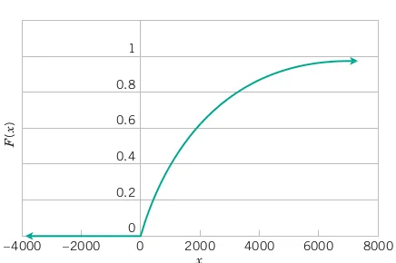
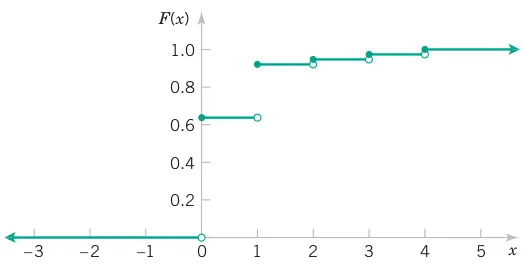
A graph of F(x) is shown in Figure 3.6. Note that F(x)=0 for x \leq 0. Also, F(x) increases to 1 as mentioned. The following probabilities should be compared to the results in previous Example.
Determine the probability that the distance until the first surface flaw is greater than 1000 micrometers.
\begin{align*} P(X > 1000) &= 1- P(X < 1000) = 1- F(1000) \\ &= 1- \left(1- e^{-1000/2000} \right) = e^{-1/2}\\ &\approx 0.6065. \end{align*}
Thus, the proportion of disks where the distance to the first flaw is greater than 1000 micrometers is approximately 0.6065.
Determine the probability that the distance is between 1000 and 2000 micrometers.
\begin{align*} P(1000 \leq X \leq 2000) &= F(2000) - F(1000) \\ &= \left(1- e^{-2000/2000} \right) - \left(1- e^{-1000/2000} \right)\\ &= e^{-1/2} - e^{-1}\\ &= 0.6065 - 0.3679 \\ &= 0.2386. \end{align*}
Therefore, the proportion of parts with a flaw distance between 1000 and 2000 micrometers is approximately 0.2386.
[1] 0.6065307[1] 0.2386512cdf1 <- function(x) {1 - exp(-x/2000)}
1 - cdf1(1000)
cdf1(2000) - cdf1(1000)Suppose X is a continuous random variable with pdf f(x). The mean or expected value of X, denoted as \mu or E(X), is
\mu = E(X) = \int_{-\infty}^{\infty} xf(x)\,dx.
The variance of X, denoted as V(X) or \sigma^{2}, is
\sigma^{2} = V(X) = \int_{-\infty}^{\infty} (x-\mu)^{2}f(x)\,dx = E(X^2) - \mu^{2}.
The standard deviation of X is \sigma.
For the distance to a flaw in the previous example, the mean of X is
\begin{align*} E(X) & = \int_{-\infty}^{\infty} x f(x)\,dx = \int_{0}^{\infty} x \frac{e^{-x/2000}}{2000}\,dx \\ & = \left[ -xe^{-x/2000} \right]_{0}^{\infty} + \int_{0}^{\infty} \frac{e^{-x/2000}}{2000}\,dx \\ E(X) & = 0 - \left[ 2000 e^{-x/2000} \right]_{0}^{\infty} = 2000. \end{align*}
The variance of X is
\begin{align*} V(X) & = \int_{-\infty}^{\infty} (x-\mu)^2 f(x)\,dx = \int_{0}^{\infty} (x-2000)^2 \frac{e^{-x/2000}}{2000}\,dx \\ V(X) & = 2000^2 = 4,000,000. \end{align*}
[1] 2000[1] 4000000Mean1 <- function(x) {x*(1/2000) * exp(-x/2000)}
integrate(
f = Mean1
, lower = 0
, upper = Inf
)$value
options(scipen = 999)
Variance1 <- function(x) {(x-2000)^2*(1/2000) * exp(-x/2000)}
integrate(
f = Variance1
, lower = 0
, upper = Inf
)$valueUndoubtedly, the most widely used model for the distribution of a random variable is a normal distribution.
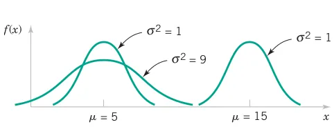
A random variable X with probability density function
\begin{align*} f\left(X\right)=\frac{1}{\sqrt{2\pi\sigma^{2}}}\exp\left\{ -\frac{1}{2}\left(\frac{X-\mu}{\sigma}\right)^{2}\right\} . \end{align*}
has a normal distribution (and is called a normal random variable) with parameters \mu and \sigma, where -\infty < \mu < \infty and \sigma > 0. Also
E(X) = \mu \quad \text{and} \quad V(X) = \sigma^2
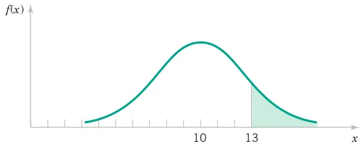
Assume that the current measurements in a strip of wire follow a normal distribution with a mean of 10 milliamperes and a variance of 4 \text{milliamperes}^2. What is the probability that a measurement exceeds 13 milliamperes?
Let X denote the current in milliamperes. The requested probability can be represented as P(X > 13). This probability is shown as the shaded area under the normal probability density function in Figure 3.8. Unfortunately, there is no closed-form expression for the integral of a normal pdf, and probabilities based on the normal distribution are typically found numerically or from a table.
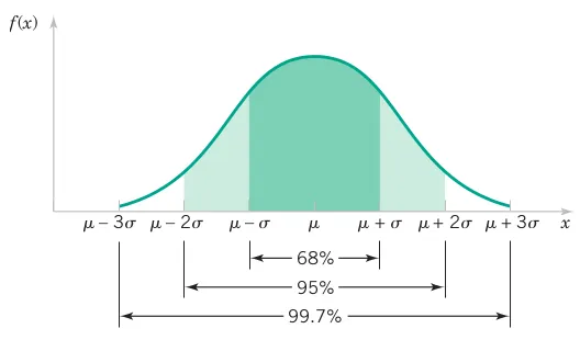
\begin{align*} P(\mu - \sigma < X < \mu + \sigma) & = 0.6827\\ P(\mu - 2\sigma < X < \mu + 2\sigma) & = 0.9545\\ P(\mu - 3\sigma < X < \mu + 3\sigma) & = 0.9973\\ \end{align*}
[1] 0.6826895[1] 0.9544997[1] 0.9973002pnorm(q = 1, mean = 0, sd = 1, lower.tail = TRUE, log.p = FALSE) -
pnorm(q = -1, mean = 0, sd = 1, lower.tail = TRUE, log.p = FALSE)
pnorm(q = 2, mean = 0, sd = 1, lower.tail = TRUE, log.p = FALSE) -
pnorm(q = -2, mean = 0, sd = 1, lower.tail = TRUE, log.p = FALSE)
pnorm(q = 3, mean = 0, sd = 1, lower.tail = TRUE, log.p = FALSE) -
pnorm(q = -3, mean = 0, sd = 1, lower.tail = TRUE, log.p = FALSE)A normal random variable with \mu = 0 and \sigma^2 = 1 is called a standard normal random variable. A standard normal random variable is denoted as Z.
The function \Phi(z) = P(Z \leq z)
is used to denote the cumulative distribution function of a standard normal random variable. A table (or computer software) is required because the probability cannot be calculated in general by elementary methods.
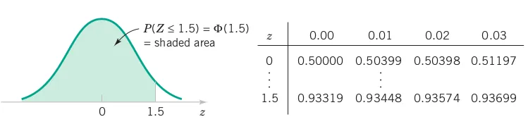
The following calculations are shown pictorially in Figure 3.12.
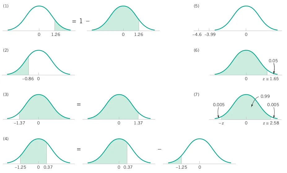
[1] 0.1038347[1] 0.1038347[1] 0.1948945[1] 0.9146565[1] 0.9146565[1] 0.538659[1] 0.000002112455[1] 1.644854[1] 2.5758291 - pnorm(q = 1.26, mean = 0, sd = 1, lower.tail = TRUE, log.p = FALSE)
pnorm(q = 1.26, mean = 0, sd = 1, lower.tail = FALSE, log.p = FALSE)
pnorm(q = -0.86, mean = 0, sd = 1, lower.tail = TRUE, log.p = FALSE)
1 - pnorm(q = -1.37, mean = 0, sd = 1, lower.tail = TRUE, log.p = FALSE)
pnorm(q = -1.37, mean = 0, sd = 1, lower.tail = FALSE, log.p = FALSE)
pnorm(q = 0.37, mean = 0, sd = 1, lower.tail = TRUE, log.p = FALSE) -
pnorm(q = -1.25, mean = 0, sd = 1, lower.tail = TRUE, log.p = FALSE)
pnorm(q = -4.6, mean = 0, sd = 1, lower.tail = TRUE, log.p = FALSE)
qnorm(p = 0.05, mean = 0, sd = 1, lower.tail = FALSE, log.p = FALSE)
qnorm(p = 0.995, mean = 0, sd = 1, lower.tail = TRUE, log.p = FALSE)If X is a normal random variable with E(X) = \mu and V(X) = \sigma^2, the random variable Z = \frac{X-\mu}{\sigma}
is a normal random variable with E(Z ) = 0 and V(Z ) = 1. That is, Z is a standard normal random variable.
Suppose X is a normal random variable with mean \mu and variance \sigma^2. Then
P\left(X \leq x\right) = P\left(\frac{X-\mu}{\sigma} \leq \frac{x-\mu}{\sigma}\right) = P\left(Z \leq z\right) where Z is a standard normal random variable, and and z = \frac{x-\mu}{\sigma} is the z-value obtained by standardizing x. The probability is obtained by entering Appendix A Table I (Figure 3.11) with z = \frac{x-\mu}{\sigma}.
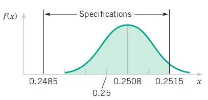
The diameter of a shaft in a storage drive is normally distributed with mean 0.2508 inch and standard deviation 0.0005 inch. The specifications on the shaft are 0.2500 \pm 0.0015 inch. What proportion of shafts conforms to specifications?
Let X denote the shaft diameter in inches. The requested probability is shown in Figure 3.13 and \begin{align*} P\left(0.2485 < X < 0.2515\right) & = P\left(\frac{0.2485-0.2508}{0.0005} \leq \frac{0.2515-0.2508}{0.0005}\right)\\ &= P\left(-4.6< Z < 1.4\right) = P\left(Z < 1.4\right) -P\left(Z < -4.6\right)\\ &= 0.91924-0.00000=0.91924 \end{align*}
[1] 0.9192412pnorm(q = 0.2515, mean = 0.2508, sd = 0.0005, lower.tail = TRUE, log.p = FALSE) -
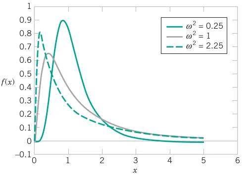
pnorm(q = 0.2485, mean = 0.2508, sd = 0.0005, lower.tail = TRUE, log.p = FALSE)Let W have a normal distribution with mean \theta and variance \omega^{2}. Then X=\exp\left(W\right) is a lognormal random variable with probability density function
f\left(x\right)=\frac{1}{x\sqrt{2\pi\omega^{2}}}\exp\left\{ -\frac{1}{2}\left(\frac{\ln\left(x\right)-\theta}{\omega}\right)^{2}\right\} \quad\text{for}\quad0<x<\infty
The mean and variance of X are E\left(X\right)=\exp\left(\theta+\frac{1}{2}\omega^{2}\right) and V\left(X\right)=\exp\left(2\theta+\omega^{2}\right)\left\{ \exp\left(\omega^{2}\right)-1\right\} respectively.
The lifetime of a semiconductor laser has a lognormal distribution with \theta = 10 and \omega = 1.5 hours. What is the probability the lifetime exceeds 10,000 hours? What lifetime is exceeded by 99% of lasers? Determine the mean and variance of lifetime.
The random variable X is the lifetime of a semiconductor laser. From the cumulative distribution function for X
\begin{align*} P\left(X > 10,000\right) & = 1- P\left(X < 10,000\right)\\ & = 1- P\left(\exp(W) < 10,000\right)\\ & = 1- P\left(W < \ln(10,000) \right)\\ & = 1- P\left(\frac{W-\theta}{\omega} < \frac{\ln(10,000)-10}{1.5} \right)\\ P\left(X > 10,000\right)&= 1- \Phi\left(-0.52 \right) = 1 - 0.30 = 0.70 \end{align*} Now the question is to determine x such that P(X>x) = 0.99. Therefore,
\begin{align*} P\left(X > x\right) & = 1- P\left(X < x\right)\\ & = 1- P\left(\exp(W) < x\right)\\ & = 1- P\left(W < \ln(x) \right)\\ & = 1- P\left(\frac{W-\theta}{\omega} < \frac{\ln(x)-10}{1.5} \right)\\ &= 0.99 \end{align*} From Figure 3.11, 1 - \Phi(z) = 0.99 when z = -2.33. Therefore, \frac{\ln(x)-10}{1.5} = -2.3263 and x = \exp(6.5105) \approx 672.5\, \text{hours}.
The mean of lifetime is \begin{align*} E\left(X\right)&=\exp\left(\theta+\frac{1}{2}\omega^{2}\right)\\ E\left(X\right)& = \exp\left(10+\frac{1}{2}\times1.5^{2}\right) = 67,846.3 \end{align*} The variance of lifetime is \begin{align*} V\left(X\right)&=\exp\left(2\theta+\omega^{2}\right)\left\{ \exp\left(\omega^{2}\right)-1\right\}\\ & = \exp\left(2\times10+1.5^{2}\right)\left\{ \exp\left(1.5^{2}\right)-1\right\}\\ V\left(X\right)& = 39,070,059,886.6 \end{align*}
[1] 0.7007086[1] 672.1478[1] 672.1478[1] 67846.29[1] 390700598871 - plnorm(q = 10000, meanlog = 10, sdlog = 1.5, lower.tail = TRUE, log.p = FALSE)
qlnorm(p = 0.99, meanlog = 10, sdlog = 1.5, lower.tail = FALSE, log.p = FALSE)
qlnorm(p = 0.01, meanlog = 10, sdlog = 1.5, lower.tail = TRUE, log.p = FALSE)
exp(10 + (1.5^2) / 2)
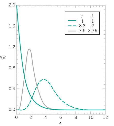
exp(2*10 + 1.5^2)*(exp(1.5^2)-1)The random variable X with probability density function f\left(x\right)=\frac{\lambda^{r}x^{r-1}\exp\left(-\lambda x\right)}{\Gamma\left(r\right)}\quad\text{for}\quad x>0
is a gamma random variable with shape parameter r>0 and rate parameter \lambda>0. \Gamma\left(r\right) is the gamma function defined as: \Gamma\left(r\right)=\int_{0}^{\infty} x^{r-1} \exp(-x)\,dx, for r>0. The mean and variance of X are E\left(X\right)=\frac{r}{\lambda} and V\left(X\right)=\frac{r}{\lambda^{2}} respectively.
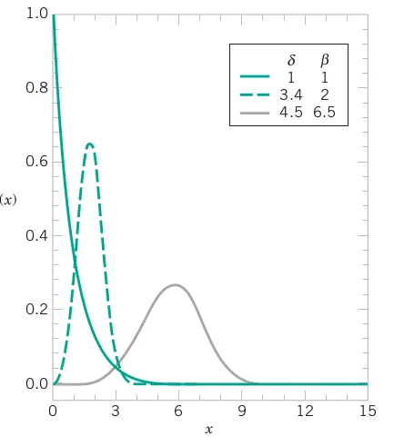
The random variable X with probability density function f\left(x\right)=\frac{\beta}{\delta}\left(\frac{x}{\delta}\right)^{\beta-1}\exp\left\{ -\left(\frac{x}{\delta}\right)^{\beta}\right\} \quad\text{for}\quad x>0
is a Weibull random variable with scale parameter \delta>0 and shape parameter \beta>0.
If X has a Weibull distribution with parameters \delta>0 and \beta>0, the cumulative distribution function of X is
F\left(x\right)=1 - \exp\left\{ -\left(\frac{x}{\delta}\right)^{\beta}\right\}
The mean and variance of X are E\left(X\right)=\delta\Gamma\left(1+\frac{1}{\beta}\right) and V\left(X\right)=\delta^{2}\Gamma\left(1+\frac{2}{\beta}\right)-\delta^{2}\left\{ \Gamma\left(1+\frac{1}{\beta}\right)\right\} ^{2} respectively.
The time to failure (in hours) of a bearing in a mechanical shaft is satisfactorily modeled as a Weibull random variable with $= $ and \delta=5000 hours. Determine the mean time until failure. Determine the probability that a bearing lasts at least 6000 hours.
The mean time until failure is \begin{align*} E\left(X\right)&=\delta\Gamma\left(1+\frac{1}{\beta}\right)\\ &=5000\times\Gamma\left(1+2\right)\\ &= 5000\times2! = 10,000 \, \text{hours} \end{align*} The probability that a bearing lasts at least 6000 hours is
\begin{align*} P\left(X > 6000\right)&= 1- F\left(6000\right)\\ &=\exp\left\{ -\left(\frac{6000}{5000}\right)^{1.5}\right\}\\ &= 0.334\\ \end{align*} Consequently, only 33.4% of all bearings last at least 6000 hours.
[1] 10000[1] 0.33439075000*gamma(1+1/0.5)
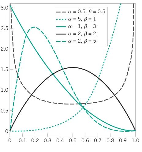
1 - pweibull(q = 6000, shape = 0.5, scale = 5000, lower.tail = TRUE, log.p = FALSE)The random variable X with probability density function f\left(x\right)=\frac{\Gamma\left(\alpha+\beta\right)}{\Gamma\left(\alpha\right)\Gamma\left(\beta\right)}x^{\alpha-1}\left(1-x\right)^{\beta-1}\quad\text{for}\quad0\leq x\leq1
is a beta random variable with parameters \alpha>0 and \beta>0. The mean and variance of X are E\left(X\right)=\frac{\alpha}{\alpha+\beta}
and V\left(X\right)=\frac{\alpha\beta}{\left(\alpha+\beta\right)^{2}\left(\alpha+\beta+1\right)} respectively.
Consider the completion time of a large commercial development. The proportion of the maximum allowed time to complete a task is modeled as a beta random variable with \alpha=2.5 and \beta=1. What is the probability that the proportion of the maximum time exceeds 0.7? Calculate the mean and variance of this random variable.
Suppose X denotes the proportion of the maximum time required to complete the task. The probability is
\begin{align*} P\left(X>0.7\right)&=\int_{0.7}^{1} \frac{\Gamma\left(\alpha+\beta\right)}{\Gamma\left(\alpha\right)\Gamma\left(\beta\right)}x^{\alpha-1}\left(1-x\right)^{\beta-1}\,dx\\ & = \int_{0.7}^{1} \frac{\Gamma\left(2.5+1\right)}{\Gamma\left(2.5\right)\Gamma\left(1\right)}x^{2.5-1}\left(1-x\right)^{1-1}\,dx\\ & = \int_{0.7}^{1} \frac{\Gamma\left(3.5\right)}{\Gamma\left(2.5\right)\Gamma\left(1\right)}x^{1.5}\,dx\\ & = \frac{2.5(1.5)(0.5)\sqrt{\pi}}{(1.5)(0.5)\sqrt{\pi}} \frac{1}{2.5} x^{2.5} \bigg|_{0.7}^{1}\\ P\left(X>0.7\right)&= 1 - 0.7^{2.5} = 0.59 \end{align*}
The mean is
\begin{align*} E\left(X\right)&=\frac{\alpha}{\alpha+\beta}\\ & = \frac{2.5}{2.5+1} = 0.71 \end{align*}
and \begin{align*} V\left(X\right)&=\frac{\alpha\beta}{\left(\alpha+\beta\right)^{2}\left(\alpha+\beta+1\right)}\\ &=\frac{2.5\times1}{\left(2.5+1\right)^{2}\left(2.5+1+1\right)}\\ & = 0.045 \end{align*}
[1] 0.5900366[1] 0.7142857[1] 0.045351471- pbeta(q = 0.7, shape1 = 2.5, shape2 = 1, ncp = 0, lower.tail = TRUE, log.p = FALSE)
2.5/(2.5 + 1)
(2.5 * 1)/((2.5 + 1)^2 * (2.5 + 1 + 1))The analysis of the surface of a semiconductor wafer records the number of particles of contamination that exceed a certain size. Define the random variable X to equal the number of particles of contamination. The possible values of X are integers from 0 up to some large value that represents the maximum number of these particles that can be found on one of the wafers. If this maximum number is very large, it might be convenient to assume that any integer from zero to is possible.
For a discrete random variable X with possible values x_{1},x_{2},\ldots,x_{n}, the probability mass function (or PMF) is
f(x_{i})=P(X=x_{i})
Because f(xi) is defined as a probability,
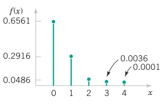
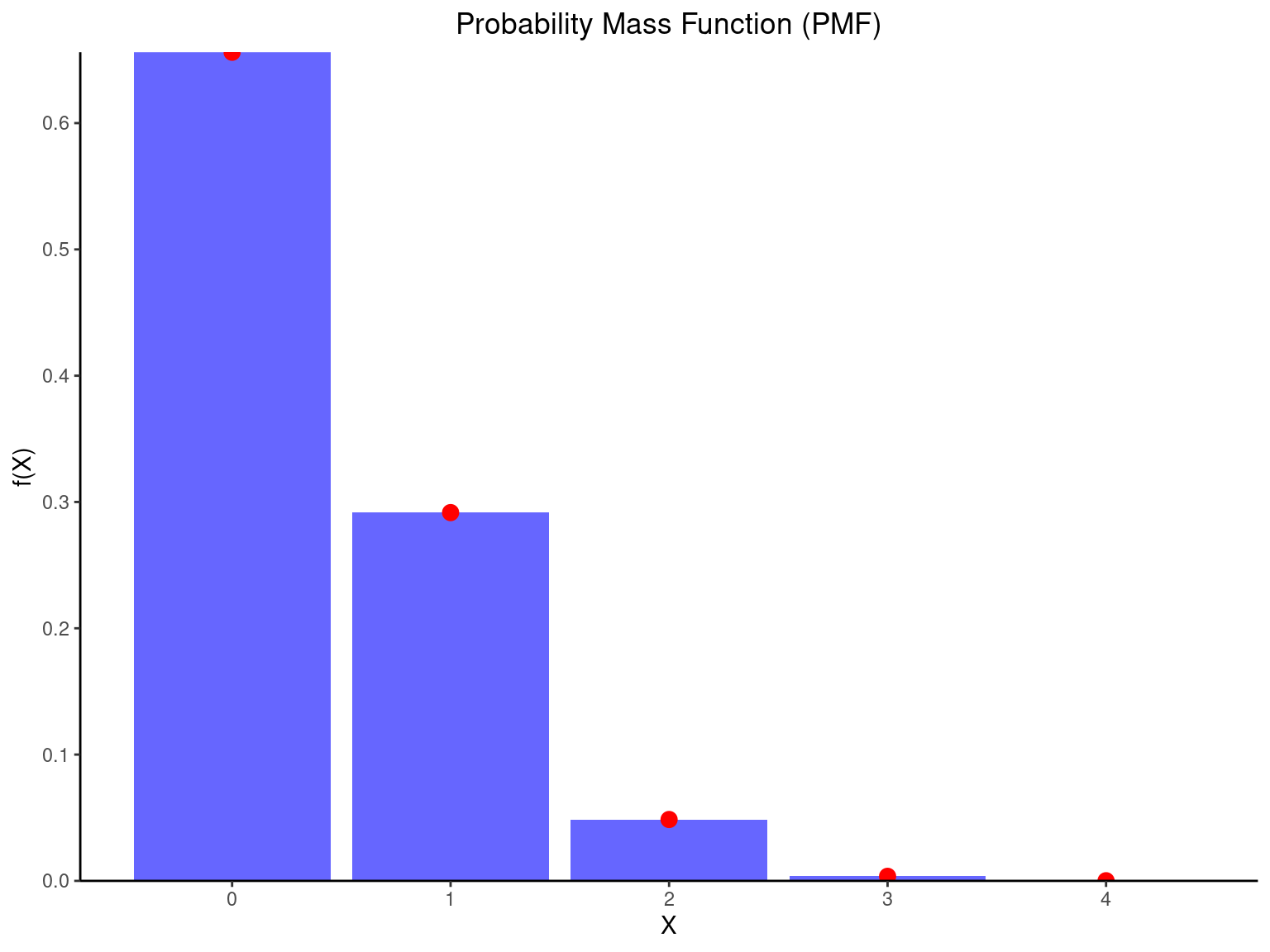
There is a chance that a bit transmitted through a digital transmission channel is received in error. Let X equal the number of bits in error in the next 4 bits transmitted. The possible values for X are {0, 1, 2, 3, 4}. Based on a model for the errors that is presented in the following section, probabilities for these values will be determined. Suppose that the probabilities are P(X = 0) = 0.6561, P(X = 1) = 0.2916, P(X = 2) = 0.0486, P(X = 3) = 0.0036, P(X = 4) = 0.0001.
The probability distribution of X is specified by the possible values along with the probability of each. A graphical description of the probability distribution of X is shown in Figure 3.18.
library(fastverse)
library(tidyverse)
library(scales)

df3 <-
  data.table(
    X  = c(0, 1, 2, 3, 4)
  , Px = c(0.6561, 0.2916, 0.0486, 0.0036, 0.0001)
  )

ggplot(data = df3, mapping = aes(x = X, y = Px)) +
  geom_bar(stat = "identity", fill = "blue", alpha = 0.6) +
  geom_point(color = "red", size = 3) +
  scale_y_continuous(expand = c(0, 0), limits = c(0, NA), breaks = pretty_breaks(n = 8)) +
  labs(
    title = "Probability Mass Function (PMF)"
  ,  x = "X"
  , y = "f(X)"
  ) +
  theme_classic() +
theme(plot.title = element_text(hjust = 0.5))The cumulative distribution function of a discrete random variable X is
F(x)=P(X\leq x)=\sum_{x_{i}\leq x}f(x_{i})
In the previous example, the probability mass function of X is
P(X = 0) = 0.6561, P(X = 1) = 0.2916, P(X = 2) = 0.0486, P(X = 3) = 0.0036, P(X = 4) = 0.0001.
Therefore, F(0) = 0.6561, F(1) = 0.6561 + 0.2916 = 0.9477, F(2) = 0.6561 + 0.2916 + 0.0486 = 0.9963, F(3) = 0.9999, F(4) = 1
Even if the random variable can assume only integer values, the cdf is defined at noninteger values. For example, F(1.5) = P(X \le 1.5) = P(X \le 1) = 0.9477
The graph of F(x) is shown in Figure 3.19. Note that the graph has discontinuities (jumps) at the discrete values for X. It is a piecewise continuous function. The size of the jump at a point x equals the probability at x. For example, consider x = 1. Here F(1) = 0.9477, but for 0 \le x < 1, F(x) = 0.6561. The change is P(X = 1) = 0.2916.
       X     Px     Fx
   <num>  <num>  <num>
1:     0 0.6561 0.6561
2:     1 0.2916 0.9477
3:     2 0.0486 0.9963
4:     3 0.0036 0.9999
5:     4 0.0001 1.0000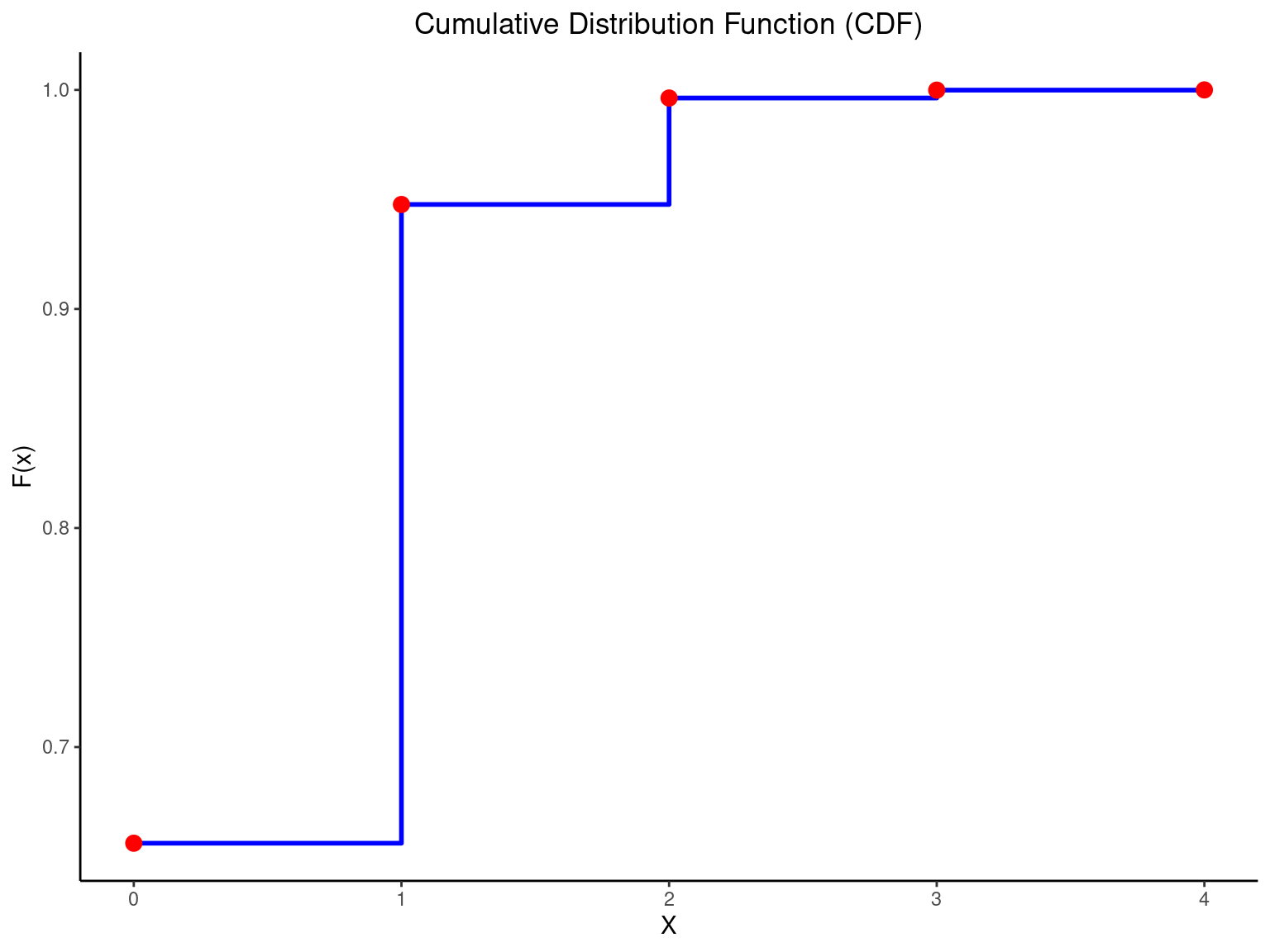
library(fastverse)
library(tidyverse)
library(scales)

df3 <-
  data.table(
    X  = c(0, 1, 2, 3, 4)
  , Px = c(0.6561, 0.2916, 0.0486, 0.0036, 0.0001)
  )

df4 <-
  df3 %>%
  fmutate(Fx = cumsum(Px))

df4
ggplot(data = df4, mapping = aes(x = X, y = Fx)) +
  geom_step(direction = "hv", color = "blue", linewidth = 1) +
  geom_point(color = "red", size = 3) +
  labs(
    title = "Cumulative Distribution Function (CDF)"
  , x     = "X"
  , y     = "F(x)"
  ) +
  theme_classic() +
theme(plot.title = element_text(hjust = 0.5))Let the possible values of the random variable X be denoted x_{1},x_{2},\ldots,x_{n}. The pmf of X is f(x), so f(x_{i})=P(X=x_{i}).
The mean or expected value of the discrete random variable X, denoted as \mu or E(X), is
\mu=E(X)=\sum_{i=1}^{n}x_{i}f(x_{i})
The variance of X, denoted as \sigma^2 or V(X), is
\begin{align*} \sigma^{2} & =V\left(X\right)=E\left(X-\mu\right)^{2}\\ \sigma^{2} & =\sum_{i=1}^{n}\left(x_{i}-\mu\right)^{2}f\left(x_{i}\right) = \sum_{i=1}^{n}x_{i}^{2}f\left(x_{i}\right) - \mu^2 \end{align*}
The standard deviation of X is \sigma.
For the number of bits in error in the previous example,
\begin{align*} \mu & =E\left(X\right)=0f(0)+1f(1)+2f(2)+3f(3)+4f(4)\\ & =0(0.6561) + 1(0.2916) + 2(0.0486) + 3(0.0036) + 4(0.0001)\\ & = 0.4 \end{align*}
Although X never assumes the value 0.4, the weighted average of the possible values is 0.4.
| x | x-0.4 | (x-0.4)^2 | f(x) | (x-0.4)^2f(x) |
|---|---|---|---|---|
| 0 | -0.4 | 0.16 | 0.6561 | 0.104976 |
| 1 | 0.6 | 0.36 | 0.2916 | 0.104976 |
| 2 | 1.6 | 2.56 | 0.0486 | 0.124416 |
| 3 | 2.6 | 6.76 | 0.0036 | 0.024336 |
| 4 | 3.6 | 12.96 | 0.0001 | 0.001296 |
V(X) = \sigma^2 = \sum_{i=1}^{n}\left(x_{i}-0.4\right)^{2}f\left(x_{i}\right) = 0.36
[1] 0.4[1] 0.36library(fastverse)
library(tidyverse)
library(scales)
df3 <-
data.table(
X = c(0, 1, 2, 3, 4)
, Px = c(0.6561, 0.2916, 0.0486, 0.0036, 0.0001)
)
df3 %>%
fmutate(XPx = X*Px) %>%
pull(XPx) %>%
fsum(x = .)
df3 %>%
fmutate(V1 = (X-0.4)^2*Px) %>%
pull(V1) %>%
fsum(x = .)Two new product designs are to be compared on the basis of revenue potential. Marketing feels that the revenue from design A can be predicted quite accurately to be $3 million. The revenue potential of design B is more difficult to assess. Marketing concludes that there is a probability of 0.3 that the revenue from design B will be $7 million, but there is a 0.7 probability that the revenue will be only $2 million. Which design would you choose?
Let X denote the revenue from design A. Because there is no uncertainty in the revenue from design A, we can model the distribution of the random variable X as $3 million with probability one. Therefore, E(X ) = \$3 million.
Let Y denote the revenue from design B. The expected value of Y in millions of dollars is E(Y ) = \$7(0.3) + \$2(0.7) = \$3.5
Because E(Y) exceeds E(X), we might choose design B. However, the variability of the result from design B is larger. That is, \begin{align*} \sigma^2 &= (7-3.5)^{2}(0.3) + (2 - 3.5)^{2}(0.7)\\ \sigma^2 & = 5.25\, \text{millions of dollars squared} \end{align*}
and \sigma = \sqrt{5.25} = 2.29\, \text{millions of dollars}
A random experiment consisting of n repeated trials such that 1. the trials are independent, 2. each trial results in only two possible outcomes, labeled as success and failure, and 3. the probability of a success on each trial, denoted as p, remains constant
is called a binomial experiment.
The random variable X that equals the number of trials resulting in a success has a binomial distribution with parameters p and p where 0\leq p\leq1 and n=\left\{ 1,2,3,\ldots,\right\}.
The PMF of X is f\left(x\right)=\binom{n}{x}p^{x}\left(1-p\right)^{n-x}\,\text{for}\,x=0,1,\ldots,n where {n \choose x}=C_{x}^{n}=\frac{n!}{x!\left(n-x\right)!}.
If X is a binomial random variable with parameters n and p, then
\mu=E\left(X\right)=np and \sigma^{2}=V\left(X\right)=np\left(1-p\right)
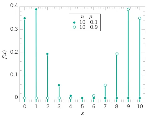
Each sample of water has a 10% chance of containing high levels of organic solids. Assume that the samples are independent with regard to the presence of the solids. Determine the probability that in the next 18 samples, exactly 2 contain high solids. Determine the probability that at least four samples contain high solids. Determine, the probability that 3 \le X \le 7. Determine, the mean and variance of X.
Let X = the number of samples that contain high solids in the next 18 samples analyzed. Then X is a binomial random variable with p = 0.1 and n = 18. Therefore,
P\left(X = 2\right)=\binom{18}{2}(0.1)^{2}\left(1-0.1\right)^{18-2} = 0.284
\begin{align*} P\left(X \ge 4 \right) & =\sum_{x=4}^{18}\binom{18}{x}(0.1)^{x}\left(1-0.1\right)^{18-x} \\ P\left(X \ge 4 \right) & = 1- P\left(X < 4 \right)\\ & = 1 - \sum_{x=0}^{3}\binom{18}{x}(0.1)^{x}\left(1-0.1\right)^{18-x} \\ & = 1 - [0.150 + 0.300 + 0.284 + 0.168]\\ P\left(X \ge 4 \right) = 0.098 \end{align*}
And
\begin{align*} \mu & = E\left(X\right)=np\\ \mu & = 4\times0.1=0.4 \end{align*}
\begin{align*} \sigma^{2}&=V\left(X\right)=np\left(1-p\right)\\ \sigma^{2}&= 4\times0.1\times0.9=0.36 \end{align*}
[1] 0.2835121[1] 153[1] 0.09819684[1] 0.09819684[1] 0.09819684[1] 0.09819684[1] 1.8[1] 1.62dbinom(x = 2, size = 18, prob = 0.1)
choose(n = 18, k = 2)
sum(dbinom(x = 4:18, size = 18, prob = 0.1))
1 - sum(dbinom(x = 0:3, size = 18, prob = 0.1))
1 - pbinom(q = 3, size = 18, prob = 0.1)
pbinom(q = 3, size = 18, prob = 0.1, lower.tail = FALSE)
18*0.1
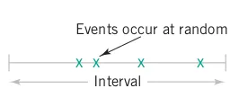
18*0.1*(1-0.1)Consider e-mail messages that arrive at a mail server on a computer network. This is an example of events (such as message arrivals) that occur randomly in an interval (such as time). The number of events over an interval (such as the number of messages that arrive in 1 hour) is a discrete random variable that is often modeled by a Poisson distribution. The length of the interval between events (such as the time between messages) is often modeled by an exponential distribution. These distributions are related; they provide probabilities for different random variables in the same random experiment. Figure 3.21 provides a graphical summary.
In general, consider an interval T of real numbers partitioned into subintervals of small length \Delta t and assume that as \Delta t tends to zero,
A random experiment with these properties is called a Poisson process.
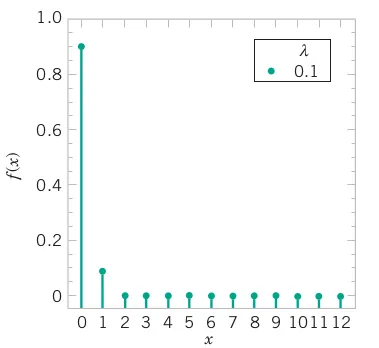
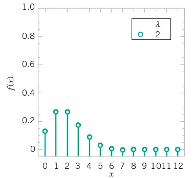
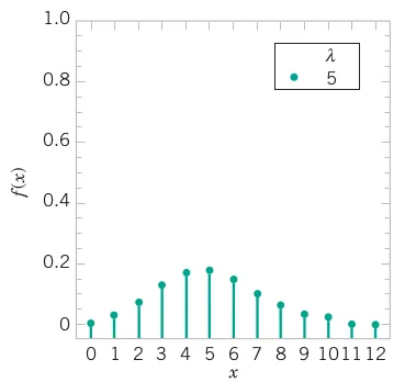
The random variable X that equals the number of events in a Poisson process is a Poisson random variable with parameter \lambda>0, and the probability mass function of X is
f\left(x\right)=\frac{\lambda^{x}\exp\left(-\lambda\right)}{x!}\quad\quad x=0,1,2,\ldots The mean and variance of X are E\left(X\right)=\lambda
and V\left(X\right)=\lambda respectively.
For the case of the thin copper wire, suppose that the number of flaws follows a Poisson distribution with a mean of 2.3 flaws per millimeter. Determine the probability of exactly 2 flaws in 1 millimeter of wire.
Let X denote the number of flaws in 1 millimeter of wire. Then X has a Poisson distribution and E(X ) = 2.3 flaws and
P(X = 2) = \frac{\exp(-2.3)\times 2.3^2}{2!} = 0.265
Determine the probability of 10 flaws in 5 millimeters of wire.
Let X denote the number of flaws in 5 millimeter of wire. Then X has a Poisson distribution with E(X) = 5 \,\text{mm} \times 2.3 \, \text{flaws/mm} = 11.5\, \text{flaws}
Therefore,
P(X = 10) = \frac{\exp(-11.5)\times 11.5^10}{10!} = 0.113
[1] 0.2651846[1] 0.1129351dpois(x = 2, lambda = 2.3)
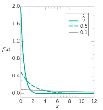
dpois(x = 10, lambda = 11.5)The random variable X that equals the distance between successive events of a Poisson process with mean \lambda>0 has an exponential distribution with parameter \lambda.
The probability distribution function of X is given by f\left(x\right)=\lambda\exp\left(-\lambda x\right)\quad\quad\text{for}\quad0\leq x<\infty
The cumulative distribution function of X is given by F\left(x\right)=1-\exp\left(-\lambda x\right)
The mean and variance of X are E\left(X\right)=\frac{1}{\lambda}
and V\left(X\right)=\frac{1}{\lambda^{2}} respectively.
In a large corporate computer network, user log-ons to the system can be modeled as a Poisson process with a mean of 25 log-ons per hour. What is the probability that there are no log-ons in an interval of 6 minutes?
Let X denote the time in hours from the start of the interval until the first log-on. Then X has an exponential distribution with \lambda = 25 log-ons per hour. We are interested in the probability that X exceeds 6 minutes. Because is given in log-ons per hour, we express all time units in hours; that is, 6 minutes = 0.1 hour. Therefore,
\begin{align*} P\left(X>0.1\right) & = \int_{0.1}^{\infty} 25\exp(-25x)\,dx \\ P\left(X>0.1\right) & = \exp\left(-25(0.1)\right) = 0.082 \end{align*}
[1] 0.082085[1] 0.082085pexp(q = 0.1, rate = 25, lower.tail = FALSE)
1 - pexp(q = 0.1, rate = 25) If X is a binomial random variable, Z = \frac{X-np}{\sqrt{np(1-p)}} is approximately a standard normal random variable. Consequently, probabilities computed from Z can be used to approximate probabilities for X.
The normal approximation to the binomial distribution is good if n is large enough relative to p, in particular, whenever
np>5\quad\text{and}\quad n\left(1-p\right)>5
A correction factor (known as a continuity correction) can be used to further improve the approximation.
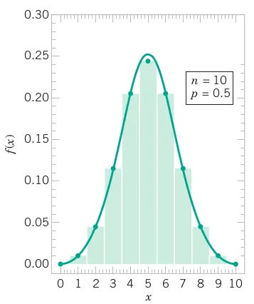
Again consider the transmission of bits in the previous example. To judge how well the normal approximation works, assume that only n = 50 bits are to be transmitted and that the probability of an error is p = 0.1. The exact probability that 2 or fewer errors occur is
\begin{align*} P(X \le 2) & = \binom{50}{0} 0.9^{50} + \binom{50}{1} 0.1(0.9^{49}) + \binom{50}{2} 0.1^{2}(0.9^{48}) \\ & = 0.11 \end{align*} Based on the normal approximation,
\begin{align*} P\left(X<2\right) & \approx P\left(Z \le \frac{2.5 - 5}{\sqrt{50(0.1)(0.9)}}\right) \\ & = P\left(Z \le -1.18\right) = 0.12 \end{align*}
[1] 0.1117288[1] 0.1192964sum(dbinom(x = 0:2, size = 50, prob = 0.1))
pnorm(q = 2.5, mean = 5, sd = sqrt(50*0.1*0.9), lower.tail = TRUE, log.p = FALSE)If X is a Poisson random variable with E(X)=\lambda and V(X)=\lambda,
Z = \frac{X-\lambda}{\sqrt{\lambda}} is approximately a standard normal random variable. Consequently, probabilities computed from Z can be used to approximate probabilities for X.
The normal approximation to the poisson distribution is good if
\lambda > 5
A correction factor (known as a continuity correction) can be used to further improve the approximation.
Assume that the number of contamination particles in a liter water sample follows a Poisson distribution with a mean of 1000. If a sample is analyzed, what is the probability that fewer than 950 particles are found?
This probability can be expressed exactly as
P(X<950) = \sum_{x=0}^{950}\frac{\exp(-1000)\times 1000^{x}}{x!} The computational difficulty is clear. The probability can be approximated as
\begin{align*} P\left(X<950\right) & \approx P\left(Z \le \frac{950.5 - 1000}{\sqrt{1000}}\right) \\ & = P\left(Z \le -1.57\right) = 0.059 \end{align*}
[1] 0.05783629[1] 0.05875308sum(dpois(x = 0:950, lambda = 1000))
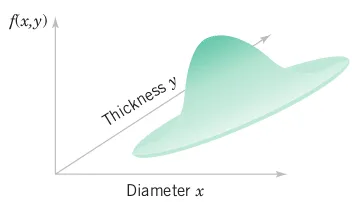
pnorm(q = 950.5, mean = 1000, sd = sqrt(1000), lower.tail = TRUE, log.p = FALSE)In many experiments, more than one variable is measured. For example, suppose both the diameter and thickness of an injection-molded disk are measured and denoted by X and Y, respectively.
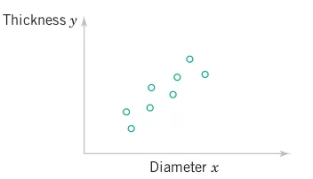
Because f(x, y) determines probabilities for two random variables, it is referred to as a joint probability density function.
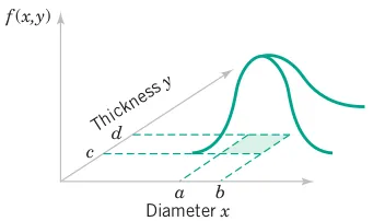
From Figure 3.27, the probability that a part is produced in the region shown is
P\left( a < X < b,\, c < Y < d\right) = \int_{a}^{b} \int_{c}^{d}f(x,y)\,dx\,dy
Similar concepts can be applied to discrete random variables.
The random variables X_1, X_2, \ldots , X_n are independent if
P(X_1 \in E_1, X_2 \in E_2, \ldots , X_n \in E_n) = P(X_1 \in E_1)P(X_2 \in E_2) \ldots P(X_n \in E_n)
for any sets E_1, E_2, \ldots , E_n.
The diameter of a shaft in a storage drive is normally distributed with mean 0.2508 inch and standard deviation 0.0005 inch. The specifications on the shaft are 0.2500 \pm 0.0015 inch. The probability that a diameter meets specifications is determined to be 0.919. What is the probability that 10 diameters all meet specifications, assuming that the diameters are independent?
Denote the diameter of the first shaft as X_1, the diameter of the second shaft as X_2, and so forth, so that the diameter of the tenth shaft is denoted as X_{10}. The probability that all shafts meet specifications can be written as
P(0.2485 < X_{1} < 0.2515, 0.2485 < X_{2} < 0.2515, \ldots , 0.2485 < X_{10} < 0.2515)
If the random variables are independent, the proportion of times in which we measure 10 shafts that we expect all to meet the specifications is
P(0.2485 < X_{1} < 0.2515) \times P(0.2485 < X_{2} < 0.2515) \times \ldots \times P(0.2485 < X_{10} < 0.2515) = 0.919^{10} = 0.430
The system shown here operates only if there is a path of functional components from left to right. The probability that each component functions is shown in the diagram. Assume that the components function or fail independently. What is the probability that the system operates?
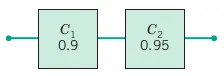
Let C_{1} and C_{2} denote the events that components 1 and 2 are functional, respectively. For the system to operate, both components must be functional. The probaility that the system operates is P(C_{1},C_{1}) = P(C_{1})P(C_{2}) = (0.9)(0.95) = 0.855
Let X be a random variable (either continuous or discrete) with mean \mu and variance \sigma^{2}, and let c be a constant. Define a new random variable Y as
Y = X + c Then
E(Y) = E(X + c) = E(X) + E(c) = \mu + c
and
V(Y) = V(X + c) = V(X) + V(c) = \sigma^{2} + 0 = \sigma^{2}
The mean and variance of the linear function of independent random variables are
\begin{align*} Y &= c_{0} + c_{1}X_{1} + c_{2}X_{2} + \ldots + c_{n}X_{n} \\ E(Y) &= c_{0} + c_{1}\mu_{1} + c_{2}\mu_{2} + \ldots + c_{n}\mu_{n} \\ V(Y) &= c_{1}^{2}\sigma_{1}^{2} + c_{2}^{2}\sigma_{2}^{2} + \ldots + c_{n}^{2}\sigma_{n}^{2} \end{align*}
Let X_{1}, X_{2}, \ldots, X_{n} be independent, normally distributed random variables with means E(X_{i}) = \mu_{i}, \, i = 1,2,\ldots, n and variances V(X_{i}) = \sigma_{i}^{2}, \, i = 1,2,\ldots, n. Then the linear function
Y = c_{0} + c_{1}X_{1} + c_{2}X_{2} + \ldots + c_{n}X_{n}
is normally distributed with mean
E(Y) = c_{0} + c_{1}\mu_{1} + c_{2}\mu_{2} + \ldots + c_{n}\mu_{n}
and variance
V(Y) = c_{1}^{2}\sigma_{1}^{2} + c_{2}^{2}\sigma_{2}^{2} + \ldots + c_{n}^{2}\sigma_{n}^{2}
Suppose that the length X_{1} and the width X_{2} are normally and independently distributed with \mu_{1} = 2 centimeters, \sigma_{1}^{2} = 0.1 centimeter, \mu_{2} = 5 centimeters, and \sigma_{2}^{2} = 0.2 centimeter. The perimeter of the part Y = 2X_{1} + 2X_{2} is just a linear combination of the length and width were E(Y) = 14 centimeters and V(Y ) = 0.2 square centimeter, respectively. Determine the probability that the perimeter of the part exceeds 14.5 centimeters.
Since Y is also a normally distributed random variable, so we may calculate the desired probability as follows:
P\left(Y>14.5\right) = P\left(\frac{Y-\mu_{Y}}{\sigma_{Y}} > \frac{14.5-14}{0.447}\right) = P\left(Z>1.12\right) = 0.13
Therefore, the probability is 0.13 that the perimeter of the part exceeds 14.5 centimeters.
The correlation between two random variables X_{1} and X_{2} is
\rho_{X_{1}X_{2}} = \frac{E\left\{(X_{1}-\mu_{1})(X_{2}-\mu_{2})\right\}}{\sqrt{\sigma_{1}^{2}\sigma_{2}^{2}}} = \frac{Cov(X_{1}, X_{2})}{\sqrt{\sigma_{1}^{2}\sigma_{2}^{2}}} with -1 \le \rho_{X_{1}X_{2}} \le +1, and \rho_{X_{1}X_{2}} is usually called the correlation coefficient.
Let X_{1}, X_{2}, \ldots, X_{n} be random variables with means E(X_{i}) = \mu_{i}, \, i = 1,2,\ldots, n and covariances Cov(X_{i}, X_{j}), \, i,j = 1,2,\ldots, n with i<j. Then the mean of the linear combination
Y = c_{0} + c_{1}X_{1} + c_{2}X_{2} + \ldots + c_{n}X_{n}
is
E(Y) = c_{0} + c_{1}\mu_{1} + c_{2}\mu_{2} + \ldots + c_{n}\mu_{n}
and the variance is
V(Y) = c_{1}^{2}\sigma_{1}^{2} + c_{2}^{2}\sigma_{2}^{2} + \ldots + c_{n}^{2}\sigma_{n}^{2} + 2 \sum_{i<j}\sum c_{i} c_{j}Cov(X_{i}, X_{j})
If X has mean \mu_{X} and variance \sigma_{X}^{2}, the approximate mean and variance of Y = h(X) can be computed using the following result:
\begin{align*} E\left(Y\right) & = \mu_{Y} = \simeq h\left(\mu_{X}\right)\\ V\left(Y\right) & = \sigma_{Y}^{2} = \simeq \left( \frac{dh}{dX}\right)^{2} \sigma_{X}^{2} \end{align*} \tag{3.1}
Engineers usually call Equation 3.1 the transmission of error or propagation of error formula.
The power P dissipated by the resistance R in an electrical circuit is given by P=I^{2}R where I, the current, is a random variable with mean \mu_{I} = 20 amperes and standard deviation \sigma_{I} = 0.1 amperes. The resistance R = 80 ohms is a constant. We want to find the approximate mean and standard deviation of the power. In this problem the function P = h(I) = I^{2}R, so taking the derivative dh/dI = 2IR = 2I(80) = 160I, we find that the approximate mean power is
\begin{align*} E\left(P\right) & = \mu_{P} \simeq h\left(\mu_{I}\right) \\ & = 20^{2}(80) = 32,000 \, \text{watts} \end{align*} and the approximate variance of power is
\begin{align*} V\left(P\right) & = \sigma_{P}^{2} \simeq \left( \frac{dh}{dX}\right)^{2} \sigma_{Y}^{2} \\ & = \left\{106(20)\right\}^{2}(0.1^2) = 102,400 \, \text{square watts} \end{align*}
Let
Y = h\left(X_{1}, X_{2}, \ldots, X_{n}\right) for independent random variables X_{i}, \, i = 1,2, \ldots, n each with mean \mu_{i} and variance \sigma_{i}^{2}, the approximate mean and variance of Y = h\left(X_{1}, X_{2}, \ldots, X_{n}\right) are
\begin{align*} E\left(Y\right) & = \mu_{Y} = \simeq h\left(\mu_{1}, \mu_{2}, \ldots, \mu_{n}\right)\\ V\left(Y\right) & = \sigma_{Y}^{2} = \simeq \sum_{i=1}^{n}\left( \frac{dh}{dX_{i}}\right)^{2} \sigma_{i}^{2} \end{align*}
Independent random variables X_{1}, X_{2}, \ldots, X_{n} with the same distribution are called a random sample.
A statistic is a function of the random variables in a random sample.
The probability distribution of a statistic is called its sampling distribution.
If X_{1}, X_{2}, \ldots, X_{n} is a random sample of size n taken from a population with mean \mu and variance \sigma^2, and if \overline{X} is the sample mean, the limiting form of the distribution of
Z = \frac{\overline{X} - \mu}{\sigma/\sqrt{n}} as n \rightarrow \infty, is the standard normal distribution.
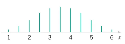
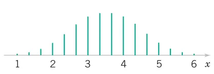
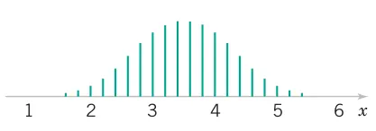
An electronics company manufactures resistors that have a mean resistance of 100 \Omega and a standard deviation of 10 \Omega. Find the probability that a random sample of n = 25 resistors will have an average resistance less than 95 \Omega.
\begin{align*} P\left(\overline{X} < 95 \right) & = P\left(\frac{\overline{X} - \mu}{\sigma/\sqrt{n}} < \frac{95 - 100}{10/\sqrt{25}} \right) \\ P\left(\overline{X} < 95 \right) & = P\left(Z < -2.5 \right) = 0.00062 \end{align*}