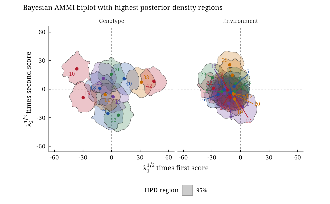
bayes_gge() fits the sites regression (SREG) model behind the GGE biplot by the method of Perez-Elizalde et
al. (2012): it is bayes_ammi(.model = "SREG"), under the name used by the package
bayesstability. The genotype main effect is part of the multiplicative terms; an earlier trial enters as
prior through .prior_data.
Usage
bayes_gge(
  .data,
  .y,
  .gen,
  .env,
  .rep,
  .nIter = 1000L,
  .prior_data = NULL,
  .n0 = NULL,
  .k = NULL,
  .burnin = 0L,
  .thin = 1L,
  .chains = 1L,
  .priors = bys_priors(),
  .level = 0.95,
  .seed = NULL,
  .align = TRUE,
  .waic = TRUE
)

# Default S3 method
bayes_gge(
  .data,
  .y,
  .gen,
  .env,
  .rep,
  .nIter = 1000L,
  .prior_data = NULL,
  .n0 = NULL,
  .k = NULL,
  .burnin = 0L,
  .thin = 1L,
  .chains = 1L,
  .priors = bys_priors(),
  .level = 0.95,
  .seed = NULL,
  .align = TRUE,
  .waic = TRUE
)
Arguments
- .data
a data frame with one row per plot.
- .y, .gen, .env, .rep
the columns of the response, genotypes, environments and replicates: bare names or strings. The same names are used in
.prior_data.- .nIter
number of iterations kept per chain before thinning (after the burn-in).
- .prior_data
NULL(default: vague priors) or a data frame of an earlier trial with the same columns, genotypes and environments, used as prior (Perez-Elizalde et al. 2012).- .n0
weight of the earlier trial: the number of its observations per cell in the prior (default its number of replicates).
- .k
number of bilinear terms \(K\) (default
NULL: all of them).- .burnin
number of iterations discarded at the start of every chain (default 0).
- .thin
keep every
.thin-th iteration (default 1).- .chains
number of chains (default 1).
- .priors
the vague priors used without an earlier trial, from
bys_priors().- .level
probability of the HPD intervals (default 0.95).
- .seed
integer seed for a reproducible run, or
NULL; the random number state of the session is restored afterwards.- .align
keep the sign of every bilinear term (default
TRUE).- .waic
compute WAIC during sampling (default
TRUE).
Value
An object of class c("bys_bayes_ammi", "bys_result", "list"); see bayes_ammi().
References
Perez-Elizalde, S., Jarquin, D. and Crossa, J. (2012). A general Bayesian estimation method of linear-bilinear models applied to plant breeding trials with genotype x environment interaction. Journal of Agricultural, Biological, and Environmental Statistics, 17(1), 15–37. doi:10.1007/s13253-011-0063-9
Author
Muhammad Yaseen (myaseen208@gmail.com)
Examples
data(cultivo2008)
data(cultivo2009)
fg <-
  bayes_gge(
      .data       = cultivo2009
    , .y          = y
    , .gen        = entry
    , .env        = site
    , .rep        = rep
    , .nIter      = 400
    , .prior_data = cultivo2008
    , .n0         = NULL
    , .k          = 2
    , .burnin     = 100
    , .thin       = 1
    , .chains     = 1
    , .priors     = bys_priors(
          mu_mean     = 0
        , mu_var      = 1e+8
        , tau_mean    = 0
        , tau_var     = 1e+8
        , delta_mean  = 0
        , delta_var   = 1e+8
        , lambda_mean = 0
        , lambda_var  = 1e+8
        , nu          = 1
        , s2          = NULL
        )
    , .level      = 0.95
    , .seed       = 1
    , .align      = TRUE
    , .waic       = TRUE
    )
fg
#> Bayesian SREG with 2 multiplicative term(s), an earlier trial as prior (n0 = 3): 12 genotypes, 25 environments, 3 replicates
#> 1 chain(s) x 400 kept draws (iterations 400 after a burn-in of 100, thinning 1); 0.3 s
#>
#> Posterior means, standard deviations and 95% HPD intervals
#>     parameter       mean        sd      lower      upper   ess
#>        <char>      <num>     <num>      <num>      <num> <num>
#>  1:        mu    3849.45     29.76    3787.60    3902.00   400
#>  2:    sigma2 1690978.83 100810.22 1503446.43 1884445.42   400
#>  3:  delta[1]     121.19    149.04    -166.23     408.42   400
#>  4:  delta[2]    -524.26    149.61    -815.78    -232.48   400
#>  5:  delta[3]     871.36    146.84     593.90    1142.31   533
#>  6:  delta[4]    -373.87    151.40    -634.37     -59.13   468
#>  7:  delta[5]    1537.40    154.45    1225.81    1817.17   322
#>  8:  delta[6]    -109.83    153.05    -407.29     158.38   340
#>  9:  delta[7]   -1758.98    147.78   -2038.72   -1457.79   400
#> 10:  delta[8]     347.82    153.03      62.58     634.26   636
#> 11:  delta[9]   -1459.37    147.87   -1733.45   -1176.00   400
#> 12: delta[10]    -729.16    150.74   -1015.43    -448.90   400
#> 13: delta[11]   -1207.60    144.31   -1452.51    -893.79   400
#> 14: delta[12]   -1902.59    158.57   -2226.59   -1616.13   400
#> 15: delta[13]    -979.97    151.20   -1241.10    -670.88   400
#> 16: delta[14]    -556.64    144.37    -833.95    -270.73   400
#> 17: delta[15]   -2207.20    147.11   -2510.07   -1944.10   400
#> 18: delta[16]      82.43    146.95    -238.97     340.44   400
#> 19: delta[17]     165.15    152.31    -173.94     420.68   400
#> 20: delta[18]    1850.87    146.37    1580.34    2147.34   400
#> 21: delta[19]    -864.01    153.32   -1154.53    -584.65   400
#> 22: delta[20]   -1110.67    150.46   -1387.43    -798.98   400
#> 23: delta[21]   -1627.47    160.34   -1913.66   -1313.32   473
#> 24: delta[22]    4923.60    157.91    4618.56    5201.61   400
#> 25: delta[23]    2869.84    147.19    2604.91    3156.31   469
#> 26: delta[24]     890.82    153.09     632.45    1206.48   400
#> 27: delta[25]    1751.14    161.16    1397.08    2024.66   400
#> 28: lambda[1]    6160.30    547.69    5158.97    7316.11   300
#> 29: lambda[2]    3222.78    603.55    1997.93    4251.27   339
#>     parameter       mean        sd      lower      upper   ess
#>        <char>      <num>     <num>      <num>      <num> <num>
#>
#> Scores of the bilinear terms: x$summary (blocks alpha, gamma); biplot coordinates: x$scores
#>
#> Sources: Perez-Elizalde et al. (2012); Crossa et al. (2011); Yan et al. (2000);
#> Hoff (2009); Spiegelhalter et al. (2002); Watanabe (2010). Full references:
#> bys_cite(x).
bp <-
  bayes_gge_biplot(
      fit           = fg
    , burnin        = 0
    , thin          = 1
    , pb            = 0.05
    , plot_stable   = TRUE
    , plot_unstable = TRUE
    , ncolors       = 5
    , .which        = "both"
    , .grid         = 100
    )
bp$biplot