Chapter and Example Map
The package implements the following book examples as help pages:
Examp1.3.2 |
16 |
ex124 |
fixed effect ANOVA with split-plot structure |
Examp2.2.1.7 |
42 |
ex121 |
dose hypothesis test |
Examp2.4.2.2 |
64 |
ex125 |
ML and REML variance components |
Examp2.4.3.1 |
66 |
ex127 |
BLUPs for sire effects |
Examp2.5.1.1 |
67 |
ex125 |
fixed effect estimates |
Examp2.5.2.1 |
68 |
ex125 |
linear combinations of fixed effects |
Examp2.5.3.1 |
70 |
ex125 |
confidence intervals |
Examp2.5.4.1 |
74 |
ex125 |
fixed versus mixed model intervals |
Examp2.6.1 |
76 |
ex125 |
fixed effect hypothesis tests |
Examp3.1 |
80, 84, 86 |
ex31 |
three PCV response models |
Examp3.2 |
88 |
ex32 |
weaning weight mixed model |
Examp3.3 |
88 onward |
ex33 |
longitudinal PCV mixed models |
Example 2.4.3.1
The sire random-effect example estimates a sire variance component and predicts sire effects.
  (Intercept)
1  -2.1979037
2  -0.0318874
3  -1.7434719
4   3.1587811
5   0.8691909
6  -0.8627975
The readable book targets are reproduced to rounding: mean near 13.97, sire variance near 3.685, residual variance near 3.542, and sire 4 BLUP near 3.16.
Example 2.6.1
The contrast for the Samorin versus Berenil comparison can be expressed against the fitted fixed-effect vector.
if (requireNamespace("lmerTest", quietly = TRUE)) {
  contrast_fit <- lmerTest::lmer(
    Pcv ~ dose * Drug + (1 | Region / Drug),
    data = ex125,
    REML = TRUE,
    contrasts = list(dose = "contr.SAS", Drug = "contr.SAS")
  )
  if (requireNamespace("report", quietly = TRUE)) {
    report::report(contrast_fit)
  }

  contrast <- matrix(
    c(0, 0, -1, -0.5),
    ncol = 4,
    dimnames = list("drug_difference", rownames(summary(contrast_fit)$coef))
  )

  lmerTest::contest(contrast_fit, contrast, joint = FALSE)
}
                 Estimate Std. Error df   t value     lower     upper
drug_difference -5.558333  0.6916667  5 -8.036145 -7.336319 -3.780348
                    Pr(>|t|)
drug_difference 0.0004825951
The estimate and variance match the readable book values (-5.55 and about 0.478). The p-value printed by current R is based on the same F statistic but can differ from the book because of software and reporting differences.
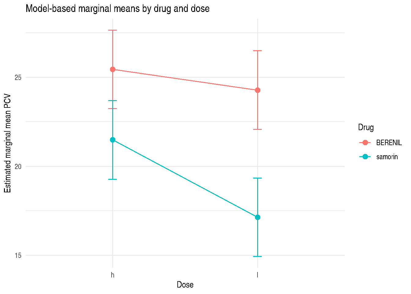
Post Hoc Inference with emmeans
After fitting a mixed model, report and emmeans provide complementary interpretations. report gives a narrative summary of the model object, while emmeans gives estimated marginal means, contrasts, and post hoc comparisons. For the split-plot example, the marginal means can be computed for dose within drug. The package helper emmeans_mixed_model() returns these same marginal means or pairwise contrasts through a guarded package-level API.
if (requireNamespace("emmeans", quietly = TRUE) && exists("contrast_fit")) {
  example_emm <- emmeans::emmeans(
    contrast_fit,
    ~ dose | Drug,
    lmer.df = "asymptotic"
  )
  example_pairs <- emmeans::contrast(example_emm, method = "pairwise")

  as.data.frame(example_emm)
} else {
  data.frame(
    workflow = "Optional marginal means",
    requirement = "Install emmeans to compute estimated marginal means"
  )
}
Drug = BERENIL:
 dose   emmean       SE  df asymp.LCL asymp.UCL
 h    25.45000 1.127996 Inf  23.23917  27.66083
 l    24.28333 1.127996 Inf  22.07250  26.49416

Drug = samorin:
 dose   emmean       SE  df asymp.LCL asymp.UCL
 h    21.48333 1.127996 Inf  19.27250  23.69417
 l    17.13333 1.127996 Inf  14.92250  19.34417

Degrees-of-freedom method: asymptotic
Confidence level used: 0.95
Drug = BERENIL:
 contrast estimate       SE  df z.ratio p.value
 h - l    1.166667 0.835946 Inf   1.396  0.1628

Drug = samorin:
 contrast estimate       SE  df z.ratio p.value
 h - l    4.350000 0.835946 Inf   5.204 <0.0001

Degrees-of-freedom method: asymptotic
if (exists("example_emm") && requireNamespace("ggplot2", quietly = TRUE)) {
  example_emm_df <- as.data.frame(example_emm)
  lower_ci <- intersect(c("lower.CL", "asymp.LCL"), names(example_emm_df))[1L]
  upper_ci <- intersect(c("upper.CL", "asymp.UCL"), names(example_emm_df))[1L]
  example_emm_df$lower_ci <- example_emm_df[[lower_ci]]
  example_emm_df$upper_ci <- example_emm_df[[upper_ci]]

  ggplot2::ggplot(
    example_emm_df,
    ggplot2::aes(x = dose, y = emmean, color = Drug, group = Drug)
  ) +
    ggplot2::geom_line(linewidth = 0.6) +
    ggplot2::geom_point(size = 2.4) +
    ggplot2::geom_errorbar(
      ggplot2::aes(ymin = lower_ci, ymax = upper_ci),
      width = 0.06,
      linewidth = 0.5
    ) +
    ggplot2::labs(
      x = "Dose",
      y = "Estimated marginal mean PCV",
      color = "Drug",
      title = "Model-based marginal means by drug and dose"
    ) +
    ggplot2::theme_minimal()
}
Modern Preprocessing Pattern
Several book examples require factor versions of design columns or indicator variables for contrasts. The package examples use a single collapse::fmutate() step so that these derived variables are readable and reproducible.
  herd animal_id PCV1 PCV2 dose    drug herd1   drug1 dose1 ber ber1 pcv_ber1
1    1       667   17   28    1 BERENIL     1 BERENIL     1   1    1       17
2    1      1003   22   23    1 BERENIL     1 BERENIL     1   1    1       22
3    1      1177   20   28    1 BERENIL     1 BERENIL     1   1    1       20
4    1       227   22   25    2 BERENIL     1 BERENIL     2   1    0        0
5    1       241   22   23    2 BERENIL     1 BERENIL     2   1    0        0
6    1       271   18   18    2 BERENIL     1 BERENIL     2   1    0        0
  pcv_ber2
1        0
2        0
3        0
4       22
5       22
6       18
Example 3.1
Example 3.1 fits increasingly rich models for packed cell volume one month after treatment. The current package data contain 38 observations, while the book page image for Model 3 shows denominator degrees of freedom greater than 300. That indicates the printed SAS output and the packaged data are not at the same observational granularity for that table. The package therefore verifies the R code logically and statistically but does not claim exact numerical agreement for the Model 3 printed table.