Power of the combining-ability tests for planning a diallel

DiallelPower() estimates by simulation the power of Griffing's \(F\) tests of gca, sca and reciprocal effects for numbers of replicates, so that the size of a diallel experiment can be planned.

Usage

DiallelPower(
  Parents,
  Method,
  Rep,
  Model = 1,
  gca,
  sca,
  rec = 0,
  Error,
  nsim = 500,
  alpha = 0.05,
  seed = NULL
)

# S3 method for class 'da_power'
plot(x, ...)

Arguments

Parents: number of parents \(P \geq 3\).
Method: Griffing's method, 1 to 4: which crosses are grown.
Rep: vector of numbers of replicates to compare.
Model: 1 (fixed effects) or 2 (random effects): which tests.
gca, sca, rec: standard deviations of the gca, sca and reciprocal effects.
Error: standard deviation of the plot errors \(\sigma\).
nsim: number of simulated data sets for each number of replicates (default 500).
alpha: level of the tests (default 0.05).
seed: seed of the random numbers, or NULL (default) to leave the generator as it is.
x: a da_power object.
...: unused.

Value

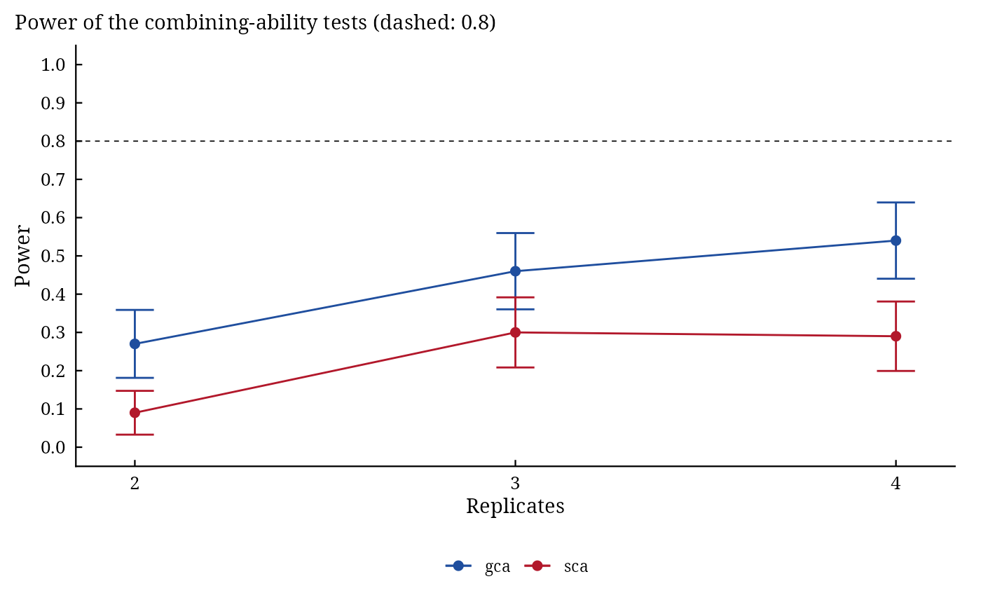
A data.table of class c("da_power", ...): columns Rep, Source (gca, sca, reciprocals), Power and SE; plot() draws the power curves.

Details

For every number of replicates in Rep, nsim data sets are drawn with DiallelSim and analysed with Griffing's closed forms; the power is the share of data sets whose test is significant at level alpha, with its Monte Carlo standard error \(\sqrt{\hat{p}(1 - \hat{p})/n_{sim}}\). The tests are those of Model: in Model 1 every line against the error, in Model 2 gca against sca. The block effects do not change the tests and are left out.

Author

Muhammad Yaseen (myaseen208@gmail.com)

Examples

pw <-
  DiallelPower(
      Parents = 6
    , Method  = 2
    , Rep     = 2:4
    , Model   = 1
    , gca     = 1
    , sca     = 1.5
    , rec     = 0
    , Error   = 4
    , nsim    = 100
    , alpha   = 0.05
    , seed    = 1
    )
pw
#>      Rep Source Power         SE
#>    <int> <char> <num>      <num>
#> 1:     2    gca  0.27 0.04439595
#> 2:     2    sca  0.09 0.02861818
#> 3:     3    gca  0.46 0.04983974
#> 4:     3    sca  0.30 0.04582576
#> 5:     4    gca  0.54 0.04983974
#> 6:     4    sca  0.29 0.04537621
plot(pw)