\(\color{green}{\textit{Sampling}}\) \(\color{green}{\textit{Design & Analysis}}\) \(\color{green}{\textit{with Applications}}\)

\(\color{green}{\textit{Muhammad Yaseen}}\)

\(\color{green}{\textit{}}\)

Introduction

Population & Sample

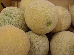
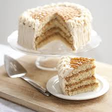
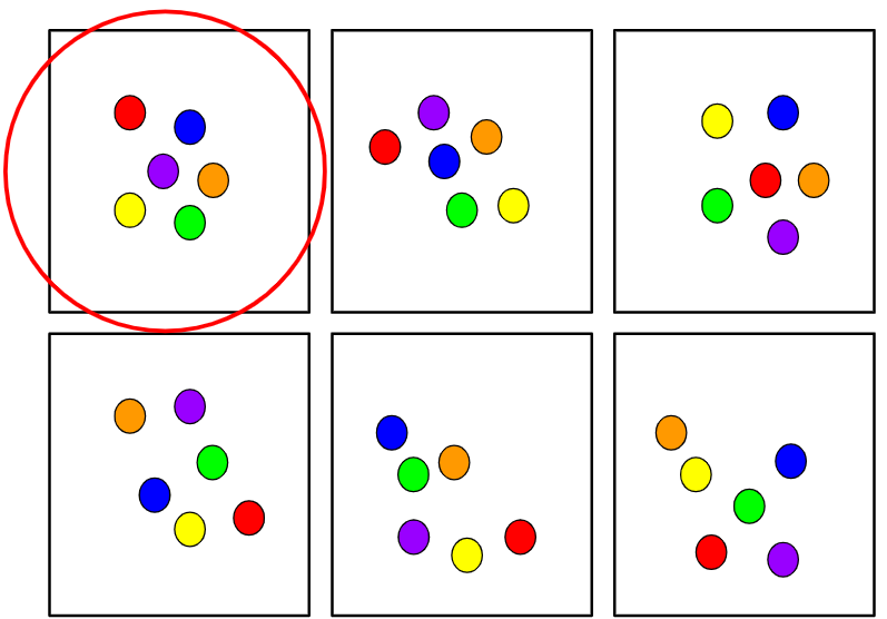
\(\color{green}{\text{Population:}}\) Totality, aggregate, whole
\(\color{green}{\text{Sample:}}\) Part or subset of totality

\(\color{green}{\text{Parameter:}}\) Value characterizing the population
\(\color{green}{\text{Statistic:}}\) Value characterizing the sample

Sampling Methods

\(\color{green}{\text{Probability Sampling:}}\) Random selection of sample allowing to make strong statistical inferences about the population

\(\color{green}{\text{Non-probability Sampling:}}\) Non-Random selection of sample based on convenience or other criteria, allowing to easily collect data

Sampling Design

\(\color{green}{\text{Sampling Design:}}\) The procedure by which the sample of units is selected from the population

\(\color{green}{\text{Sampling Frame:}}\) A list, map, or other specification of units in the population from which a sample may be selected

Probability Sampling

Each unit in the population has a known probability of selection
If implemented well, a relatively small sample can be used to make inferences about an arbitrarily large population
Examples:
- \(\color{green}{\text{Simple Random Sampling}}\)
- \(\color{green}{\text{Stratified Random Sampling}}\)
- \(\color{green}{\text{Cluster Random Sampling}}\)
- \(\color{green}{\text{Systematics Random Sampling}}\)

Framework of Probability Sampling

The finite population of \(N\) units is denoted by the index set \(\mathscr{\mathcal{U}}=\left\{ 1,2,\ldots,N\right\}\)
The particular sample of \(n\) units chosen is denoted by \(\mathscr{\mathcal{S}}\)
Each possible sample \(\mathscr{\mathcal{S}}\) from the population has a known probability \(P\mathscr{\left(\mathcal{S}\right)}\) of being chosen and \(\sum P\mathscr{\left(\mathcal{S}\right)}=1\)
Each possible sample has a known probability of being the chosen sample, each unit in the population has a known probability of appearing in our selected sample \(\pi_{i}=P\left(\text{unit }i\text{ in sample}\right)\), \(\pi_{i}\) is the probability that unit \(i\) is included in the sample.

Define the sampling weight, sometimes called the design weight, to be the reciprocal of the inclusion probability: \(w_{i}=\frac{1}{\pi_{i}}.\) The sampling weight of sampled unit \(i\) can be interpreted as the number of population units represented by unit \(i\).

Sampling Distributions

The distribution of different values of the statistic obtained by the process of taking all possible samples from the population
Want to estimate a population quantity, say the population total \(t=\sum_{i=1}^{N}y_{i}\)
One possible estimator for \(t\) is \(\widehat{t}_{\mathcal{S}}=N\overline{y}_{\mathcal{S}}\), where \(\overline{y}_{\mathcal{S}}\) is the average of the \(y_{i}\)s in \(\mathscr{\mathcal{S}}\)

The probabilities of selection for the samples give the sampling distribution of \(\widehat{t}\): \[ P\left\{ \widehat{t}=k\right\} =\sum_{\mathcal{S}:\widehat{t}_{\mathcal{S}}=k}P\left(\mathcal{S}\right)\] The summation is over all samples \(\mathscr{\mathcal{S}}\) for which \(\widehat{t}_{\mathcal{S}}=k\).

Sampling Distributions

\(\color{green}{\text{Expected Value}}\): \[E\left[\widehat{t}\right]=\sum_{\mathcal{S}}\widehat{t}_{\mathcal{S}}P\left(\mathcal{S}\right)=\sum_{k}kP\left(\widehat{t}=k\right)\]
\(\color{green}{\text{Estimation Bias}}\): \[\text{Bias}\left[\widehat{t}\right]=E\left[\widehat{t}\right]-t\] If \(\text{Bias}\left[\widehat{t}\right]=0\), the estimator \(\widehat{t}\) is unbiased for \(t\).

Sampling Distributions

\(\color{green}{\text{Variance}}\): \[V\left[\widehat{t}\right] =E\left[\left(\widehat{t}-E\left[\widehat{t}\right]\right)^{2}\right]\] \[V\left[\widehat{t}\right] =\sum_{\begin{smallmatrix}\text{all possible}\\ \text{samples }\mathcal{S} \end{smallmatrix}}P\left(\mathcal{S}\right)\left(\widehat{t}_{\mathcal{S}}-E\left[\widehat{t}\right]\right)^{2}\]
\(\color{green}{\text{Mean Squared Error}}\): \[\text{MSE}\left[\widehat{t}\right] =V\left(\widehat{t}\right)+\left[\text{Bias}\left(\widehat{t}\right)\right]^{2}\]

Sampling Distributions

An estimator \(\widehat{t}\) of \(t\) is unbiased if \(E\left[\widehat{t}\right]=t\), precise if \(V\left[\widehat{t}\right]=E\left[\left(\widehat{t}-E\left[\widehat{t}\right]\right)^{2}\right]\) is small, and accurate if \(\text{MSE}\left[\widehat{t}\right]=E\left[\left(\widehat{t}-t\right)^{2}\right]\) is small.
A badly biased estimator may be precise but it will not be accurate; accuracy (MSE) is how close the estimate is to the true value, while precision (variance) measures how close estimates from different samples are to each other.

Sampling Distributions

\(\color{green}{\text{Population Total}}\): \[t=\sum_{i=1}^{N}y_{i}\]
\(\color{green}{\text{Population Mean}}\): \[\overline{y}_{\mathcal{U}}=\frac{1}{N}\sum_{i=1}^{N}y_{i}\]

Sampling Distributions

\(\color{green}{\text{Population Variance}}\): \[S^{2}=\frac{1}{N-1}\sum_{i=1}^{N}\left(y_{i}-\overline{y}_{\mathcal{U}}\right)^{2}\]
\(\color{green}{\text{Population Proportion}}\): \[p=\frac{\text{number of units with the characteristic in the population}}{N}\]

Simple Random Sampling

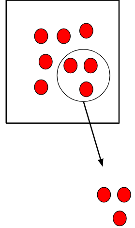
A Simple Random Sample (SRS) is the simplest form of probability sample

An SRS of size \(n\) is taken when every possible subset of \(n\) units in the population has the same chance of being the sample

SRSs are the foundation for more complex sampling designs

Stratified Random Sampling

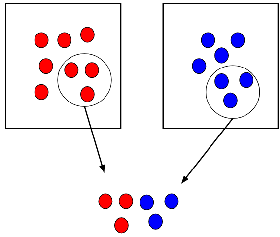
Divide the population into at least two different subgroups (or strata) that share the same characteristics

Select a SRS from each subgroup (or stratum) independently

Allocating Observations to Strata

\(\color{green}{n}\): Total Sample Size, from all Strata
\(\color{green}{n_{h}}\): Sample Size taken in Stratum \(h\)
\(\color{green}{N_{h}}\): Number of Population Units in Stratum \(h\)
\(\color{green}{S_{h}^2}\): Population Variance in Stratum \(h\)
\(\color{green}{C_{h}}\): Cost of taking an observation in Stratum \(h\)
\(\color{green}{\text{Proportional Allocation:}}\) \(n_{h}=n\times\frac{N_{h}}{\sum N_{h}}\)

Allocating Observations to Strata

\(\color{green}{n}\): Total Sample Size, from all Strata
\(\color{green}{n_{h}}\): Sample Size taken in Stratum \(h\)
\(\color{green}{N_{h}}\): Number of Population Units in Stratum \(h\)
\(\color{green}{S_{h}^2}\): Population Variance in Stratum \(h\)
\(\color{green}{C_{h}}\): Cost of taking an observation in Stratum \(h\)
\(\color{green}{\text{Neyman Allocation:}}\) \(n_{h}=n\times\frac{N_{h}\sqrt{S_{h}^{2}}}{\sum\left(N_{h}\sqrt{S_{h}^{2}}\right)}\)

Allocating Observations to Strata

\(\color{green}{n}\): Total Sample Size, from all Strata
\(\color{green}{n_{h}}\): Sample Size taken in Stratum \(h\)
\(\color{green}{N_{h}}\): Number of Population Units in Stratum \(h\)
\(\color{green}{S_{h}^2}\): Population Variance in Stratum \(h\)
\(\color{green}{C_{h}}\): Cost of taking an observation in Stratum \(h\)
\(\color{green}{\text{Optimal Allocation:}}\) \(n_{h}=n\times\frac{\frac{N_{h}\sqrt{S_{h}^{2}}}{\sqrt{C_{h}}}}{\sum\left(\frac{N_{h}\sqrt{S_{h}^{2}}}{\sqrt{C_{h}}}\right)}\)

Cluster Random Sampling

Divide the population area into sections (or clusters)

Randomly select some of those clusters

choose all the members from those selected clusters

Systematic Random Sampling

A starting point \(r\), from \(1,\ldots , k\) \(\left(k = \frac{N}{n}\right)\), is chosen from a list of population members using a random number

That unit, and every \(k\)th unit thereafter, is chosen to be in the sample

A systematic sample thus consists of units that are equally spaced in the list

Analysis

Simple Random Sampling (Population Mean)

\(\overline{y}_{\mathcal{S}}=\frac{1}{n}\sum_{i\in\mathcal{S}}y_{i}\)
\(\widehat{V\left(\overline{y}\right)}=\left(1-\frac{n}{N}\right)\frac{s^{2}}{n}\)
\(s^{2}=\frac{1}{n-1}\sum_{i\in\mathcal{S}}\left(y_{i}-\overline{y}\right)^{2}\)

\(SE\left(\overline{y}\right)=\sqrt{\left(1-\frac{n}{N}\right)\frac{s^{2}}{n}}\)

Simple Random Sampling (Population Total)

\(\widehat{t}=N\overline{y}\)
\(\widehat{V\left(\widehat{t}\right)}=N\widehat{V\left(\overline{y}\right)}=N^{2}\left(1-\frac{n}{N}\right)\frac{s^{2}}{n}\)

\(SE\left(\widehat{t}\right)=\sqrt{N^{2}\left(1-\frac{n}{N}\right)\frac{s^{2}}{n}}\)

Simple Random Sampling (Population Proportion)

\(\widehat{p}=\overline{y}\)
\(\widehat{V\left(\widehat{p}\right)}=\left(1-\frac{n}{N}\right)\frac{\widehat{p}\left(1-\widehat{p}\right)}{n-1}\)

\(SE\left(\widehat{p}\right)=\sqrt{\left(1-\frac{n}{N}\right)\frac{\widehat{p}\left(1-\widehat{p}\right)}{n-1}}\)

Stratified Random Sampling (Population Mean)

\(\overline{y}_{\text{str}}=\sum_{h=1}^{H}\frac{N_{h}}{N}\overline{y_{h}}\)
\(\widehat{V\left(\overline{y}_{\text{str}}\right)}=\sum_{h=1}^{H}\left(1-\frac{n_{h}}{N_{h}}\right)\left(\frac{N_{h}}{N}\right)^{2}\frac{s_{h}^{2}}{n_{h}}\)

\(SE\left(\overline{y}_{\text{str}}\right)=\sqrt{\sum_{h=1}^{H}\left(1-\frac{n_{h}}{N_{h}}\right)\left(\frac{N_{h}}{N}\right)^{2}\frac{s_{h}^{2}}{n_{h}}}\)

Stratified Random Sampling (Population Total)

\(\widehat{t}_{\text{str}}=\sum_{h=1}^{H}N_{h}\overline{y_{h}}\)
\(\widehat{V\left(\widehat{t}_{\text{str}}\right)}=\sum_{h=1}^{H}\left(1-\frac{n_{h}}{N_{h}}\right)N_{h}^{2}\frac{s_{h}^{2}}{n_{h}}\)

\(SE\left(\overline{y}_{\text{str}}\right)=\sqrt{\sum_{h=1}^{H}\left(1-\frac{n_{h}}{N_{h}}\right)N_{h}^{2}\frac{s_{h}^{2}}{n_{h}}}\)

Stratified Random Sampling (Population Proportion)

\(\widehat{p}_{\text{str}}=\sum_{h=1}^{H}\frac{N_{h}}{N}\widehat{p}_{h}\)
\(\widehat{V\left(\widehat{p}_{\text{str}}\right)}=\sum_{h=1}^{H}\left(1-\frac{n_{h}}{N_{h}}\right)\left(\frac{N_{h}}{N}\right)^{2}\frac{\widehat{p}_{h}\left(1-\widehat{p}_{h}\right)}{n_{h}-1}\)

\(SE\left(\widehat{p}_{\text{str}}\right)=\sqrt{\sum_{h=1}^{H}\left(1-\frac{n_{h}}{N_{h}}\right)\left(\frac{N_{h}}{N}\right)^{2}\frac{\widehat{p}_{h}\left(1-\widehat{p}_{h}\right)}{n_{h}-1}}\)

Applications

Simple Random Sampling

SRSfm1 <-
  agsrs1 |> 
  as_survey_design(
    ids          = 1
  , probs        = NULL
  , strata       = NULL
  , variables    = NULL
  , fpc          = fpc
  , nest         = FALSE
# , check_strata = !nest
  , weights      = Weight
  , pps          = FALSE
  , variance     = c("HT", "YG")
  )

Simple Random Sampling

Population Mean
- Average number of acres devoted to farms, 1992

Mean	SE	LCL	UCL	Var	CV
297897	18898.43	260706.3	335087.8	357150824	0.0634395

Population Mean
- Average number of acres devoted to farms, 1992 by Region

Region	Mean	SE	LCL	UCL	Var	CV
NC	350292.01	26985.37	297186.69	403397.33	728210378	0.0770368
NE	71970.83	12360.14	47646.95	96294.71	152772977	0.1717381
S	206246.35	23065.74	160854.60	251638.11	532028439	0.1118359
W	598680.59	77636.58	445897.25	751463.93	6027439196	0.1296795

Simple Random Sampling

Population Total
- Total number of acres devoted to farms, 1992

Total	SE	LCL	UCL	Var	CV
916927110	58169381	802453859	1031400361	3.383677e+15	0.0634395

Population Total
- Total number of acres devoted to farms, 1992 by Region

Region	Total	SE	LCL	UCL	Var	CV
NC	384557574	41022160	303828848	465286299	1.682818e+15	0.1066736
NE	17722098	4490614	8884885	26559311	2.016562e+13	0.2533907
S	275091387	35287421	205648224	344534549	1.245202e+15	0.1282753
W	239556051	46090457	148853274	330258829	2.124330e+15	0.1923995

Simple Random Sampling

Population Proportion
- Proportion of the population that falls in each of multiple categories

lt2005	Mean	SE	LCL	UCL	Var	CV
0	0.49	0.027465	0.4359508	0.5440492	0.0007543	0.0560510
1	0.51	0.027465	0.4559508	0.5640492	0.0007543	0.0538529

Population Proportion
- Total of the population that falls in each of multiple categories

lt2005	Total	SE	LCL	UCL	Var	CV
0	1508.22	84.53722	1341.857	1674.583	7146.542	0.0560510
1	1569.78	84.53722	1403.417	1736.143	7146.542	0.0538529

Simple Random Sampling

Population Proportion
- Proportion of the population that falls in each of multiple categories

Region	Mean	SE	LCL	UCL	Var	CV
NC	0.3566667	0.0263176	0.3048756	0.4084578	0.0006926	0.0737875
NE	0.0800000	0.0149051	0.0506678	0.1093322	0.0002222	0.1863138
S	0.4333333	0.0272252	0.3797561	0.4869106	0.0007412	0.0628274
W	0.1300000	0.0184768	0.0936389	0.1663611	0.0003414	0.1421295

Simple Random Sampling

Population Proportion
- Total of the population that falls in each of multiple categories

Region	Total	SE	LCL	UCL	Var	CV
NC	1097.82	81.00543	938.4070	1257.2330	6561.879	0.0737875
NE	246.24	45.87792	155.9555	336.5245	2104.784	0.1863138
S	1333.80	83.79917	1168.8891	1498.7109	7022.301	0.0628274
W	400.14	56.87169	288.2205	512.0595	3234.389	0.1421295

Stratified Random Sampling

Stratafm1 <-
  agstrat1 |> 
  as_survey_design(
    ids          = 1
  , probs        = NULL
  , strata       = region
  , variables    = NULL
  , fpc          = popsize
  , nest         = FALSE
# , check_strata = !nest
  , weights      = strwt
  , pps          = FALSE
  , variance     = c("HT", "YG")
  )

Stratified Random Sampling

Population Mean
- Average number of acres devoted to farms, 1992

Mean	SE	LCL	UCL	Var	CV
295560.8	16379.87	263325	327796.5	268300231	0.0554196

Population Mean
- Average number of acres devoted to farms, 1992 by Region

Region	Mean	SE	LCL	UCL	Var	CV
NC	300504.16	16107.59	268804.25	332204.1	259454437	0.0536019
NE	97629.81	18149.49	61911.41	133348.2	329404127	0.1859011
S	211315.04	18925.35	174069.74	248560.3	358169038	0.0895599
W	662295.51	93403.65	478476.12	846114.9	8724242692	0.1410302

Stratified Random Sampling

Population Total
- Total number of acres devoted to farms, 1992

Total	SE	LCL	UCL	Var	CV
909736035	50417248	810514350	1008957721	2.541899e+15	0.0554196

Population Total
- Total number of acres devoted to farms, 1992 by Region

Region	Total	SE	LCL	UCL	Var	CV
NC	316731380	16977399	283319676	350143084	2.882321e+14	0.0536019
NE	21478558	3992889	13620510	29336606	1.594316e+13	0.1859011
S	292037391	26154840	240564386	343510397	6.840756e+14	0.0895599
W	279488706	39416342	201916922	357060491	1.553648e+15	0.1410302

Stratified Random Sampling

Population Proportion
- Proportion of the population that falls in each of multiple categories

lt200k	Mean	SE	LCL	UCL	Var	CV
0	0.4860852	0.0247946	0.4372893	0.5348812	0.0006148	0.0510087
1	0.5139148	0.0247946	0.4651188	0.5627107	0.0006148	0.0482464

Population Proportion
- Total of the population that falls in each of multiple categories

lt200k	Total	SE	LCL	UCL	Var	CV
0	1496.17	76.31765	1345.976	1646.364	5824.383	0.0510087
1	1581.83	76.31765	1431.636	1732.024	5824.383	0.0482464

References

Cochran, W. G. (1977). Sampling Techniques. John Wiley & Sons.

Ellis , G. F., T. Lumley, T. Żółtak, et al. (2022). srvyr: ‘dplyr’-Like Syntax for Summary Statistics of Survey Data. R Package Version 1.1.1. URL: https://cran.r-project.org/web/packages/srvyr/.

Lohr, S. L. (2022). Sampling: Design and Analysis. CRC Press.

Lu, Y. and S. Lohr (2021). SDAResources: Datasets and Functions for ‘Sampling: Design and Analysis, 3rd Edition’. R Package Version 0.1.1. URL: https://cran.r-project.org/web/packages/SDAResources/.

References (Cont’d…)

Lumley, T. (2021). survey: Analysis of Complex Survey Samples. R Package Version 4.1.1. URL: https://cran.r-project.org/web/packages/survey/.

R Core Team (2022). R: A Language & Environment for Statistical Computing. R Foundation for Statistical Computing. Vienna, Austria. URL: http://www.R-project.org/.

Thompson, S. K. (2012). Sampling. John Wiley & Sons.

Tillé, Y. and A. Matei (2021). sampling: Survey Sampling. R Package Version 2.9. URL: https://cran.r-project.org/web/packages/sampling/.