Introduction to R, RStudio, and Quarto

A Beginner’s Guide to Data Analysis

M. Yaseen

School of Mathematical and Statistical Sciences
Clemson University

Welcome to Data Analysis!

Three Essential Tools:

R: Free, powerful programming language for statistics
RStudio: User-friendly interface for R
Quarto: Modern publishing system for reports

Complete Ecosystem for:

Data import and cleaning
Statistical analysis
Professional visualizations
Reproducible reports
Scientific publishing

Why These Tools Matter

Used by millions of data scientists, researchers, and analysts worldwide for everything from academic research to business intelligence.

Why Use R, RStudio, and Quarto?

Key Advantages:

Completely Free - No licensing fees ever
Beginner-Friendly - Simple commands, intuitive interfaces
Professional Results - Publication-ready outputs
Widely Used - Industry standard tools
Great Community - Extensive help and tutorials

Practical Benefits:

Reproducible Research - Share and verify analyses
Versatile Applications - From simple calculations to complex modeling
Multiple Output Formats - HTML, PDF, Word from one source
Version Control - Track changes and collaborate effectively

Bottom Line: These tools transform how you work with data, making complex analyses accessible and professional reporting automatic.

Getting Started with R

What is R?

R is Much More Than a Calculator:

Statistical Computing Environment - Built by statisticians for data analysis
Data Management System - Handle datasets of any size
Graphics Engine - Beautiful, publication-ready charts
Programming Language - Automate repetitive tasks
Statistical Toolkit - Thousands of specialized functions

What Makes R Special:

Designed for Data - Tasks difficult elsewhere are straightforward in R
Extensive Libraries - Over 19,000 packages available
Active Development - Constantly updated with latest methods
Cross-Platform - Works on Windows, Mac, Linux
Integration - Connects with databases, web APIs, other languages

Installing R

Simple 5-Step Process:

Visit Official Website - https://cran.r-project.org/
Choose Your OS - Windows, macOS, or Linux
Download Latest Version - Always get the most recent release
Run Installer - Use default settings for beginners
Verify Installation - Open R to confirm it works

Installation Tip

CRAN (Comprehensive R Archive Network) is the official and safest source. Avoid third-party downloads to ensure authentic, secure software.

Next Step: While R works alone, RStudio makes everything much easier!

Basic Math in R

# Basic operations
2 + 2

[1] 4

5 - 2

[1] 3

5 * 2

[1] 10

6 / 2

[1] 3

# Advanced functions with explicit arguments
sqrt(x = 16)

[1] 4

2^3

[1] 8

abs(x = -5)

[1] 5

round(x = 3.14159, digits = 2)

[1] 3.14

# Variables
my_age <- 25
my_height <- 170
bmi <- my_height / (my_age * 2)
cat("BMI:", bmi, "\n")

BMI: 3.4

Key Concepts:

Explicit Arguments - Use x = and digits = for clarity
Variable Assignment - Use <- to store values
Function Calls - Always include parentheses and argument names

Working with Data Tables

# Load all required packages for this tutorial
library(data.table) # Fast data manipulation and file reading
library(fastverse) # Collection of fast R packages for data science
library(tidyverse) # Collection of packages for data science workflow
library(readxl) # Read Excel files (.xlsx, .xls)
library(openxlsx) # Write Excel files and advanced Excel operations
library(knitr) # Dynamic report generation and table formatting
library(ggplot2) # Advanced data visualization (part of tidyverse)

# Create data (packages already loaded in setup-packages chunk)
students <-
  data.table(
    name = c("Alice", "Bob", "Charlie", "Diana"),
    age = c(20, 22, 21, 23),
    grade = c(85, 92, 78, 88),
    major = c("Math", "Physics", "Chemistry", "Biology")
  )

students

      name   age grade     major
    <char> <num> <num>    <char>
1:   Alice    20    85      Math
2:     Bob    22    92   Physics
3: Charlie    21    78 Chemistry
4:   Diana    23    88   Biology

str(students)

Classes 'data.table' and 'data.frame':  4 obs. of  4 variables:
 $ name : chr  "Alice" "Bob" "Charlie" "Diana"
 $ age  : num  20 22 21 23
 $ grade: num  85 92 78 88
 $ major: chr  "Math" "Physics" "Chemistry" "Biology"
 - attr(*, ".internal.selfref")=<externalptr>

Why data.table? Faster performance, intuitive syntax, memory efficient, better for beginners

Basic Statistics with Fastverse

# Basic statistics using fastverse (already loaded)
students %>%
  fsummarise(
    avg_age = fmean(age),
    avg_grade = fmean(grade),
    max_grade = fmax(grade),
    min_grade = fmin(grade)
  )

   avg_age avg_grade max_grade min_grade
     <num>     <num>     <num>     <num>
1:    21.5     85.75        92        78

# Enhanced statistics
students %>%
  fsummarise(
    n_students = fnobs(age),
    age_range = paste(fmin(age), "to", fmax(age)),
    grade_range = paste(fmin(grade), "to", fmax(grade)),
    grade_sd = round(x = fsd(grade), digits = 2)
  )

   n_students age_range grade_range grade_sd
        <int>    <char>      <char>    <num>
1:          4  20 to 23    78 to 92     5.91

Essential Statistics Explained:

Mean: Average of all values
Max/Min: Highest and lowest values
Standard Deviation: How spread out the data is
Count: Number of observations

Creating Professional Visualizations

# Create visualization (ggplot2 already loaded)
p1 <-
  ggplot(data = students, mapping = aes(x = name, y = grade, fill = major)) +
  geom_col() +
  labs(title = "Student Grades by Major", x = "Student", y = "Grade", fill = "Major") +
  theme_minimal() +
  theme(plot.title = element_text(hjust = 0.5))

# Display the plot
p1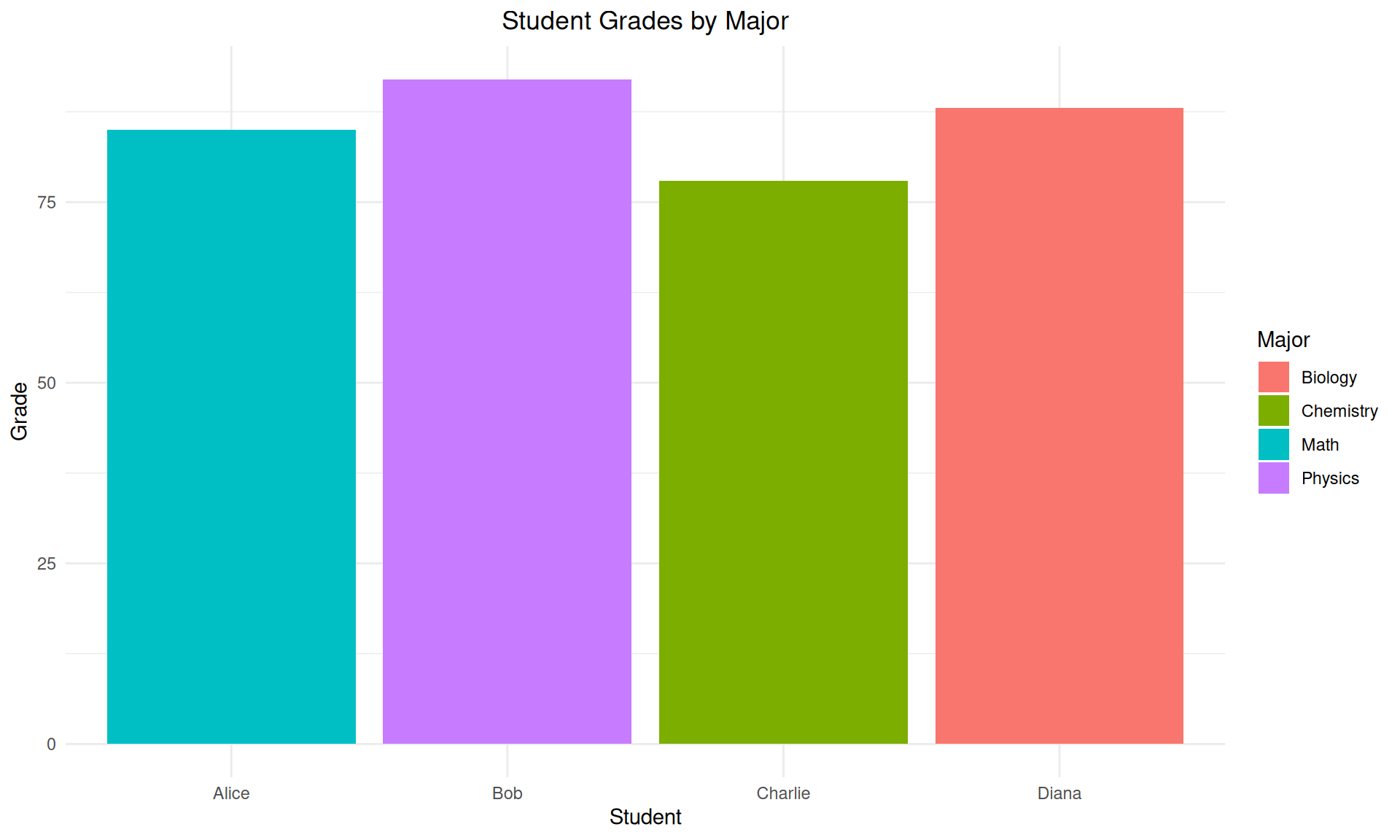

# Save the plot
ggsave(
  plot = p1,
  filename = "figures/student_grades.png",
  width = 8,
  height = 6,
  dpi = 300
)

Visualization Benefits: Patterns become immediately obvious - Bob has highest grade (92), Charlie lowest (78)

RStudio: Your R Interface

What is RStudio?

Integrated Development Environment (IDE):

RStudio transforms R from a basic command line into a professional workspace with:

Syntax Highlighting - Color-coded commands
Auto-completion - Faster, error-free coding
Project Management - Organized workflows
Integrated Help - Documentation at your fingertips

Four-Panel Layout:

Script Editor (top-left) - Write and save code
Console (bottom-left) - Interactive R commands
Environment/History (top-right) - See variables and past commands
Files/Plots/Help (bottom-right) - Navigation and outputs

Bottom Line: RStudio makes R accessible to beginners while remaining powerful for experts

Installing RStudio

Prerequisites and Steps:

Before Installing:

R Must Be Installed First - RStudio requires R to function
Check R Installation - Open R to verify it works

Installation Process:

Visit https://posit.co/downloads/
Choose RStudio Desktop (free version)
Download for your operating system
Run installer with default settings

After Installation:

Launch RStudio - You should see four-panel interface
Verify R Connection - Console should show R version
Explore Interface - Familiarize yourself with panels

First Steps:

Create a new script (File → New File → R Script)
Try typing 2 + 2 in console
Use Help panel to explore documentation

Creating and Managing Projects

# Create directories
dirs <- c("data", "figures", "R", "out")
sapply(dirs, dir.create, showWarnings = FALSE)

# Sample data (data.table already loaded)
sales <-
  data.table(
    month = c("Jan", "Feb", "Mar", "Apr", "May", "Jun"),
    sales = c(100, 120, 150, 130, 160, 180),
    region = rep(c("North", "South"), 3)
  )

# Export files (packages already loaded)
fwrite(x = sales, file = "data/sales.csv")
write.xlsx(x = sales, file = "data/sales.xlsx")

cat("Files created:\n")
list.files(path = "data", full.names = TRUE)

Why Use Projects?

Organization - Keep related files together
Working Directory - Automatic folder management
Portability - Easy sharing with collaborators
Version Control - Git integration for tracking changes

Project Benefits:

Reproducibility - Others can run your code easily
Collaboration - Share entire project folders
Backup - Everything in one place
Scalability - From simple analyses to complex research

Best Practice: Always work within projects - it saves time and prevents errors!

Introduction to Quarto

What is Quarto?

Next Generation Publishing System:

Quarto combines code, results, and narrative in professional documents:

Code Execution - Run R code automatically
Dynamic Results - Charts and tables update automatically
Professional Formatting - Publication-ready appearance
Multiple Formats - HTML, PDF, Word from one source

Reproducible Research Revolution:

Traditional Approach Problems:

Analyze in one program
Chart in another program
Write in word processor
Manually copy results (error-prone!)

Quarto Solution:

Everything in one document
Automatic updates when data changes
Complete transparency and reproducibility

Installing Quarto

Simple Installation Process:

Installation Steps:

Visit Official Site - https://quarto.org/docs/get-started/
Download Installer - Choose Windows, macOS, or Linux
Run with Defaults - Standard installation handles everything
Restart RStudio - Enables Quarto integration
Verify Installation - Look for Quarto options in menus

Integration Benefits:

Seamless RStudio Integration - New file types available
Render Buttons - One-click document creation
Preview Modes - See results while writing
Project Templates - Quick start options
Version Control - Works with Git automatically

Result: Professional document creation becomes as easy as writing an email!

Output Formats

HTML (Web Sharing)

format: html

Best for:

Interactive sharing
Online viewing
Email distribution
Web publishing

Features:

Interactive elements
Easy sharing via links
Mobile responsive
Search functionality

PDF (Professional)

format: pdf

Best for:

Academic papers
Professional reports
Print documents
Archival purposes

Features:

Page numbers
Professional typography
Print-ready quality
Consistent formatting

Word (Collaboration)

format: docx

Best for:

Team collaboration
Client reviews
Comment workflows
Non-R users

Features:

Microsoft Word compatible
Track changes support
Easy editing by others
Familiar interface

Power: Write once, publish everywhere - same content, multiple professional formats!

Complete Quarto Example

# Weather data
weather <-
  data.table(
    day = c("Mon", "Tue", "Wed", "Thu", "Fri"),
    temp = c(22, 25, 23, 27, 24),
    humidity = c(60, 55, 65, 50, 58),
    condition = c("Sunny", "Cloudy", "Rainy", "Sunny", "Partly Cloudy")
  )

# Statistics with pipe and fastverse
weather %>%
  fsummarise(
    avg_temp = fmean(temp),
    max_temp = fmax(temp),
    min_temp = fmin(temp)
  )

   avg_temp max_temp min_temp
      <num>    <num>    <num>
1:     24.2       27       22

# Create and save visualization
p2 <- ggplot(data = weather, mapping = aes(x = day, y = temp, fill = condition)) +
  geom_col() +
  labs(title = "Daily Temperature", x = "Day", y = "Temperature (°C)", fill = "Condition") +
  theme_minimal() +
  geom_text(mapping = aes(label = paste(temp, "°C")), vjust = -0.3)

# Display the plot
p2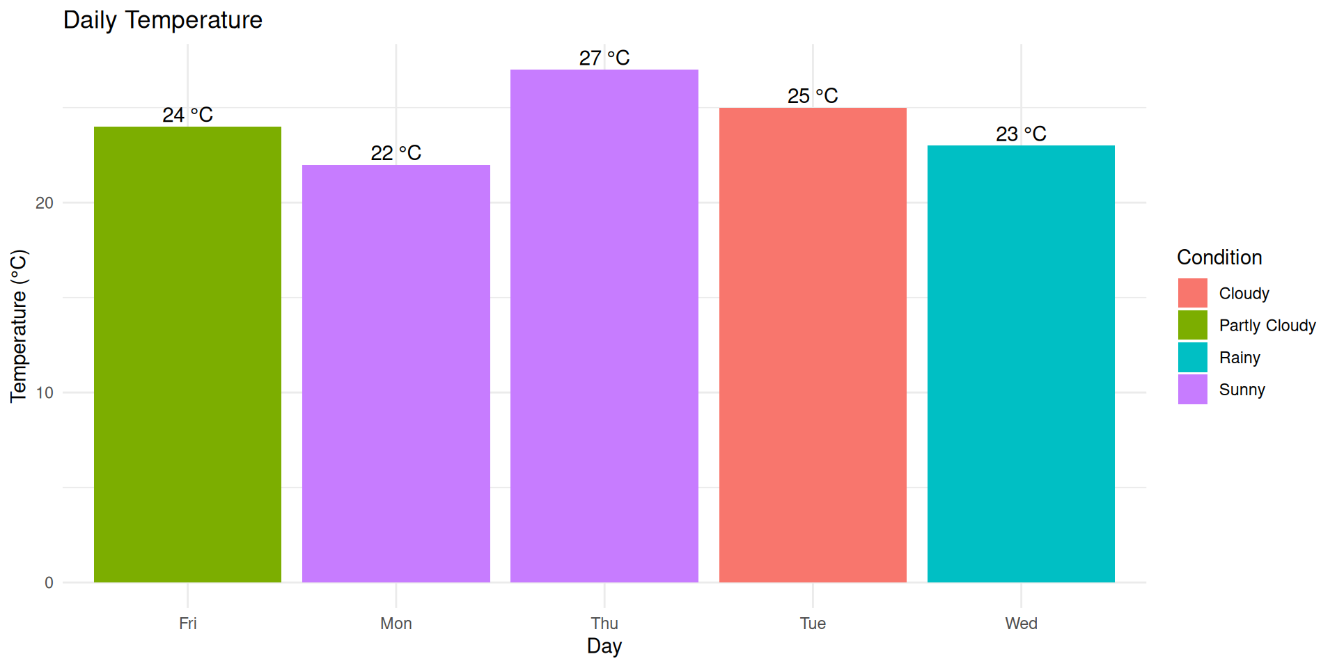

# Save the plot
ggsave(
  plot = p2,
  filename = "figures/daily_temperature.png",
  width = 10,
  height = 6,
  dpi = 300
)

Key Features Demonstrated: Automatic code execution, professional formatting, figure captioning, statistical analysis integration

Working with Data Files

Reading and Writing Data

# Read data efficiently with explicit arguments (packages already loaded)
sales_csv <- fread(file = "data/sales.csv")
sales_excel <- read_excel(path = "data/sales.xlsx") %>% as.data.table()

# Compare datasets
identical(x = sales_csv, y = sales_excel)
rbindlist(l = list(CSV = sales_csv, Excel = sales_excel), idcol = "Source")

File Format Comparison:

CSV Files - Plain text, widely compatible, smaller size
Excel Files - Multiple sheets, formatting, larger size
data.table - R-optimized, fastest performance

Why fread() over read.csv()?

Much faster performance
Better type detection
More flexible with delimiters
Cleaner handling of messy data

Best Practices:

Use relative paths - “data/file.csv” not “C:/Users/…”
Consistent naming - lowercase, underscores, descriptive
Organized folders - separate data, scripts, outputs
Backup originals - never modify raw data files

Practical Data Analysis Example

# Test scores data
scores <-
  data.table(
    student = c("Anna", "Bob", "Carol", "David", "Eva"),
    math = c(85, 92, 78, 88, 95),
    english = c(88, 85, 92, 80, 90),
    science = c(82, 90, 85, 92, 88)
  )

# Display table with knitr (already loaded)
kable(x = scores, caption = "Student Test Scores")

Student Test Scores
student	math	english	science
Anna	85	88	82
Bob	92	85	90
Carol	78	92	85
David	88	80	92
Eva	95	90	88

# Calculate subject averages using fastverse
subject_summary <-
  scores %>%
  fsummarise(
    Math = fmean(math),
    English = fmean(english),
    Science = fmean(science)
  ) %>%
  pivot(
    how = "longer",
    names = list("Subject", "Average")
  )

kable(x = subject_summary, caption = "Subject Averages", digits = 1)

Subject Averages
Subject	Average
Math	87.6
English	87.0
Science	87.4

Creating Comparison Visualizations

# Reshape data for visualization
subject_avg <-
  scores %>%
  fsummarise(
    Math    = fmean(math),
    English = fmean(english),
    Science = fmean(science)
  ) %>%
  pivot(
    how = "longer",
    names = list("Subject", "Average")
  )

# Create and save comparison chart
p3 <- ggplot(data = subject_avg, mapping = aes(x = Subject, y = Average, fill = Subject)) +
  geom_col(alpha = 0.8, show.legend = FALSE) +
  labs(title = "Average Test Scores by Subject", x = "Subject", y = "Average Score") +
  theme_minimal() +
  geom_text(mapping = aes(label = round(x = Average, digits = 1)), vjust = -0.3) +
  ylim(0, 100)

# Display the plot
p3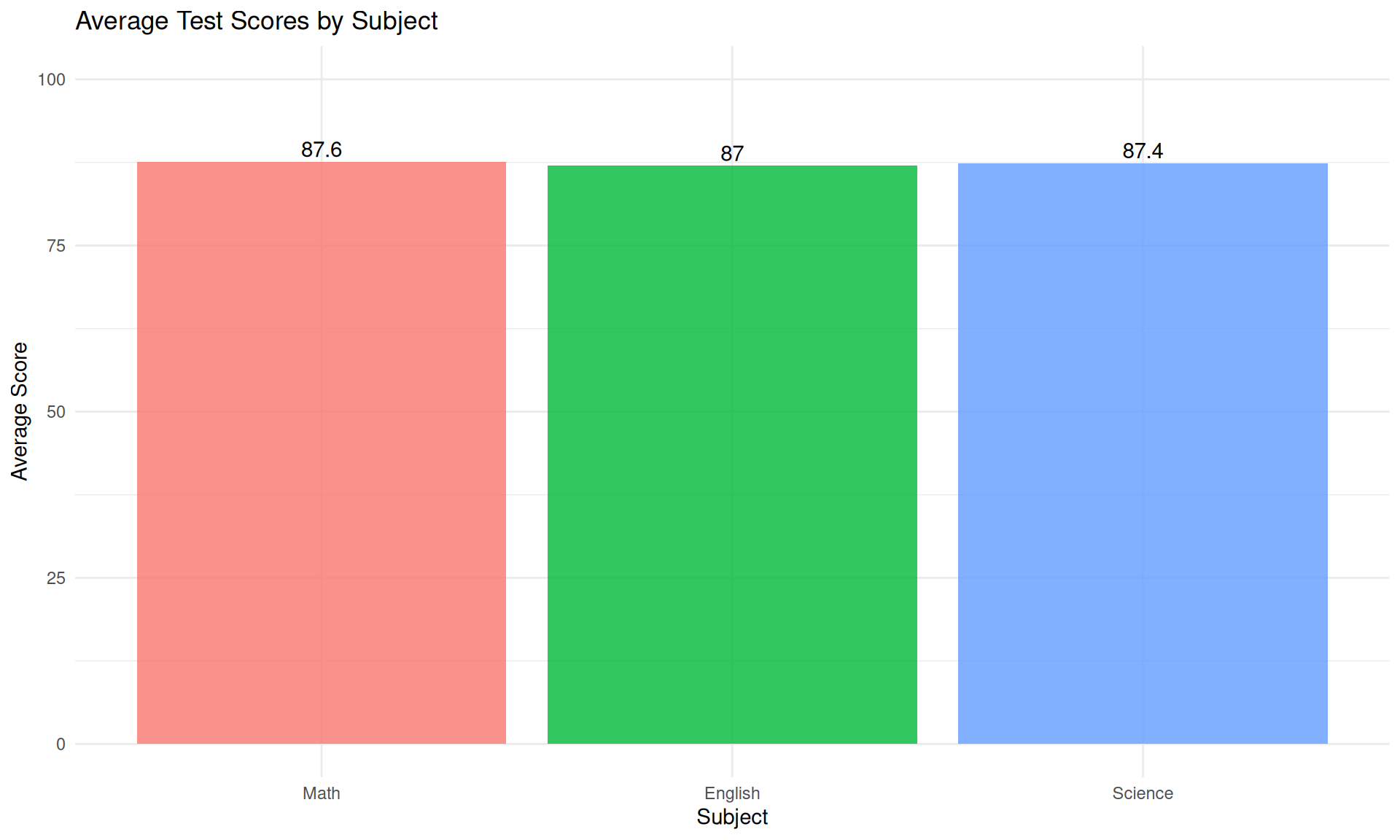

# Save the plot
ggsave(
  plot = p3,
  filename = "figures/subject_averages.png",
  width = 8,
  height = 6,
  dpi = 300
)

Insight: Visualization immediately reveals that Math scores are highest on average, demonstrating the power of charts over tables alone.

Essential Tips for Success

Getting Help When You Need It

# Help functions with explicit arguments
?mean
help.search(pattern = "regression")
example(topic = "mean")

# Package help
help(package = "data.table")

Built-in Help System:

Function Help - ?function_name for documentation
Search Help - help.search("topic") for related functions
Examples - example("function") for working code
Package Help - help(package = "packagename") for overview

External Resources:

Stack Overflow - Huge Q&A community
RStudio Community - Friendly, helpful forum
R-bloggers - Daily tutorials and tips
Local User Groups - In-person networking and learning
Documentation Sites - Official package guides

Remember: Every expert was once a beginner - the R community is known for being welcoming and helpful!

Common Mistakes and Solutions

Critical Mistakes to Avoid:

Case Sensitivity - Mean ≠ mean
Quotation Marks - Text needs quotes: "Alice"
Package Loading - Always library(package) first
Parentheses - Every ( needs a )
Explicit Arguments - Use round(x = 3.14, digits = 2)

Project Organization:

my-analysis/
├── data/           # Raw data files
├── R/              # R scripts  
├── figures/        # Generated plots
├── out/            # Output files
└── README.md       # Project description

Best Practice: Develop good habits early - they save hours of debugging later!

Keyboard Shortcuts for Efficiency

Essential Shortcuts:

Ctrl+Enter (Win) / Cmd+Enter (Mac) - Run current line
Ctrl+Shift+Enter - Run entire code chunk
Tab - Auto-complete function names
Ctrl+Z - Undo last action
Ctrl+Shift+C - Comment/uncomment lines

Navigation Shortcuts:

Ctrl+L - Clear console
Ctrl+1 - Focus on script editor
Ctrl+2 - Focus on console
Ctrl+S - Save current file
Ctrl+Shift+N - New script file

Time Saver: Master 3-4 shortcuts first, then gradually add more - they dramatically speed up your workflow!

Troubleshooting Common Issues

# If you see "packagename not found"
install.packages("packagename")
library(packagename)

install.packages("ggplot2")
library(ggplot2)

# Install multiple packages
install.packages(c("data.table", "readxl", "openxlsx"))

# Session information
sessionInfo()

Package Problems:

“Package not found” - Install first: install.packages("packagename")
Loading errors - Check package spelling and internet connection
Version conflicts - Update R and packages regularly
Missing dependencies - R usually installs these automatically

Data Import Issues:

File not found - Check file path and working directory
Encoding problems - Try encoding = "UTF-8" parameter
Wrong delimiters - Some “CSV” files use semicolons or tabs
Path problems - Use forward slashes: "data/file.csv"

Debug Strategy: Read error messages carefully, Google specific errors, check documentation, ask for help - in that order!

Conclusion and Next Steps

What You’ve Accomplished Today

Technical Skills Mastered:

✅ Installation - R, RStudio, Quarto setup
✅ Basic Operations - Math, statistics with fastverse
✅ Data Management - Creating and manipulating data.table
✅ Visualizations - Professional charts with ggplot2
✅ Reports - Dynamic documents with Quarto
✅ Best Practices - Explicit arguments, project organization

Conceptual Understanding:

✅ Reproducible Research - Code + results + narrative
✅ Modern Workflow - Projects, version control, collaboration
✅ Professional Output - Multiple formats from one source
✅ Community Resources - Help systems and support networks
✅ Troubleshooting - Independent problem-solving skills

Achievement Unlocked: You now have the foundation for modern data science!

Your Learning Journey Continues

Immediate Next Steps:

Personal Project - Analyze data you care about
Practice Explicit Arguments - Always use parameter names
Reproduce This Tutorial - Try with different data
Experiment with Styling - Modify colors and themes
Master Basic Workflow - Projects → Scripts → Reports

Skill Development Path:

Advanced ggplot2 - Scatter plots, histograms, faceting
Data Import Mastery - Excel, databases, web APIs
Statistical Methods - Regression, hypothesis testing
Advanced Quarto - Presentations, websites, books
Package Ecosystem - Specialized tools for your field

Remember: Every expert started exactly where you are now - the key is consistent practice!

Essential Learning Resources

Free Online Books:

R for Data Science (Wickham and Grolemund 2016) - The definitive beginner’s guide
Quarto Documentation - Comprehensive feature guide
ggplot2 Book (Wickham 2016) - Deep dive into visualization
fastverse Documentation - Efficient data manipulation

Interactive Learning:

RStudio Education - Free courses and tutorials
Swirl - Learn R interactively within R
DataCamp - Structured courses (some free)

Community Resources:

R-bloggers - Daily articles and tutorials
#RStats Twitter - Active community sharing tips
Local R Meetups - Network with other users
Stack Overflow - Q&A for specific problems
RStudio Community - Friendly help forum

Professional Development:

Conferences - useR!, rstudio::conf
Certification - RStudio certifications available
Specialized Training - Industry-specific workshops

Final Encouragement

You’re Joining a Global Community:

These tools are used daily by:

Data Scientists at Google, Netflix, Facebook
Researchers at universities worldwide
Analysts in government and non-profits
Students in psychology, finance, biology
Professionals in healthcare, marketing, sports

Remember:

Everyone starts as a beginner - You’re in good company
The community is welcoming - Don’t hesitate to ask for help
Practice makes progress - Consistent work beats perfection
Focus on problems you care about - Personal interest drives learning
Document your journey - Future you will thank present you

Your Mantra Going Forward

Always use explicit argument names, save your work regularly, and don’t hesitate to ask for help when you need it.

Thank You!

Key Takeaways:

Free, powerful tools for professional data analysis
Reproducible research changes how you work with data
Strong community support for continuous learning
Multiple output formats from single source documents
Modern workflow that scales from simple to complex

Contact & Resources:

Questions? Use RStudio Community forum
Advanced Help? Stack Overflow with #r tag
Stay Updated? Follow R-bloggers and #RStats
Local Community? Search for R User Groups
Official Docs? R, RStudio, and Quarto websites

Happy Analyzing! 🎉📊📈

R Packages Used

# Load all required packages for this tutorial
library(data.table) # Fast data manipulation and file reading
library(fastverse) # Collection of fast R packages for data science
library(tidyverse) # Collection of packages for data science workflow
library(readxl) # Read Excel files (.xlsx, .xls)
library(openxlsx) # Write Excel files and advanced Excel operations
library(knitr) # Dynamic report generation and table formatting
library(ggplot2) # Advanced data visualization (part of tidyverse)

Package Ecosystem Overview

data.table (Dowle and Srinivasan 2023) - High-performance data manipulation, much faster than base R data.frame

fastverse - Collection of fast, complementary packages for efficient data science workflows

tidyverse (Wickham and Grolemund 2016) - Integrated packages for data science: ggplot2, dplyr, readr, and more

readxl & openxlsx - Read and write Excel files without requiring Excel installation

knitr - Dynamic document generation and professional table formatting

ggplot2 (Wickham 2016) - Grammar of graphics for beautiful, publication-ready visualizations

References

Dowle, Matt, and Arun Srinivasan. 2023. Data.table: Extension of Data.frame. https://r-datatable.com/.

Wickham, Hadley. 2016. Ggplot2: Elegant Graphics for Data Analysis. Springer-Verlag New York. https://ggplot2.tidyverse.org.

Wickham, Hadley, and Garrett Grolemund. 2016. R for Data Science: Import, Tidy, Transform, Visualize, and Model Data. O’Reilly Media. https://r4ds.had.co.nz/.