1 Introduction

Welcome to the exciting world of data analysis! This comprehensive guide will teach you three essential tools that work together to make data analysis both powerful and accessible:

R: A free, open-source programming language specifically designed for statistics and data analysis
RStudio: A user-friendly integrated development environment (IDE) that makes working with R much easier
Quarto: A modern publishing system that allows you to create professional reports, presentations, and websites

These tools form a complete ecosystem for modern data science, allowing you to import data, analyze it, create visualizations, and share your findings in professional documents (Posit Team 2022).

1.1 Why Use These Tools?

The combination of R, RStudio, and Quarto offers several compelling advantages for beginners and professionals alike (Wickham and Grolemund 2016; Posit Team 2023):

Completely Free: All three tools are open-source and free to use, with no licensing fees or subscription costs
Beginner-Friendly: Despite their power, these tools are designed with simple commands and intuitive interfaces
Professional Results: Create publication-ready charts, statistical analyses, and formatted reports (Wickham 2016)
Widely Used: Millions of data scientists, researchers, and analysts worldwide use these tools daily
Great Community: Large, helpful community with extensive tutorials, documentation, and support
Reproducible Research: Your analysis can be easily shared and reproduced by others (Allaire et al. 2022)
Versatile: Suitable for everything from simple calculations to complex statistical modeling

2 Getting Started with R

2.1 What is R?

R is much more than just a calculator—it’s a complete statistical computing environment. Originally developed by statisticians for statisticians, R has evolved into one of the world’s most popular tools for data analysis. Think of R as:

A powerful calculator that can handle complex mathematical operations
A data management system that can work with datasets of any size
A graphics engine that creates beautiful, publication-ready charts
A programming language that can automate repetitive tasks
A statistical toolkit with thousands of specialized functions

R is particularly valuable because it’s designed specifically for working with data, making tasks that are difficult in other software surprisingly straightforward.

2.2 Installing R

Getting R installed on your computer is straightforward:

Visit the official website: Go to https://cran.r-project.org/
Choose your operating system: Click on “Download R for Windows,” “Download R for macOS,” or “Download R for Linux”
Download the latest version: Always choose the most recent version (usually at the top of the list)
Run the installer: Use default settings unless you have specific requirements
Verify installation: Open R to make sure it starts correctly

Installation Tip

The CRAN (Comprehensive R Archive Network) website is the official and safest place to download R. Avoid downloading from other websites to ensure you get an authentic, virus-free version.

2.3 Basic Math in R

Let’s start with the fundamentals. R can perform all standard mathematical operations and much more. Notice how we use clear argument names to make our code easy to understand:

# Basic operations
2 + 2

[1] 4

5 - 2

[1] 3

5 * 2

[1] 10

6 / 2

[1] 3

# Advanced functions with explicit arguments
sqrt(x = 16)

[1] 4

2^3

[1] 8

abs(x = -5)

[1] 5

round(x = 3.14159, digits = 2)

[1] 3.14

# Variables
my_age <- 25
my_height <- 170
bmi <- my_height / (my_age * 2)
cat("BMI:", bmi, "\n")

BMI: 3.4

As you can see, R can handle basic arithmetic effortlessly. The cat() function helps us display results clearly. Using explicit argument names like x = and digits = makes your code much easier to read and understand, especially when you’re learning.

2.4 Working with Data Tables

One of the most important concepts in data analysis is working with structured data. We’ll use the powerful data.table package along with fastverse and tidyverse for efficient data operations:

# Load all required packages for this tutorial
library(data.table) # Fast data manipulation and file reading
library(fastverse) # Collection of fast R packages for data science
library(tidyverse) # Collection of packages for data science workflow
library(readxl) # Read Excel files (.xlsx, .xls)
library(openxlsx) # Write Excel files and advanced Excel operations
library(knitr) # Dynamic report generation and table formatting
library(ggplot2) # Advanced data visualization (part of tidyverse)

Package Loading

All the packages we need for this tutorial are loaded in the setup chunk above. This keeps our code organized and ensures everything is available when we need it.

# Create data (packages already loaded in setup-packages chunk)
students <-
  data.table(
    name = c("Alice", "Bob", "Charlie", "Diana"),
    age = c(20, 22, 21, 23),
    grade = c(85, 92, 78, 88),
    major = c("Math", "Physics", "Chemistry", "Biology")
  )

students

      name   age grade     major
    <char> <num> <num>    <char>
1:   Alice    20    85      Math
2:     Bob    22    92   Physics
3: Charlie    21    78 Chemistry
4:   Diana    23    88   Biology

str(students)

Classes 'data.table' and 'data.frame':  4 obs. of  4 variables:
 $ name : chr  "Alice" "Bob" "Charlie" "Diana"
 $ age  : num  20 22 21 23
 $ grade: num  85 92 78 88
 $ major: chr  "Math" "Physics" "Chemistry" "Biology"
 - attr(*, ".internal.selfref")=<externalptr>

The data.table package offers several advantages over base R (Dowle and Srinivasan 2023):

Faster performance: Especially noticeable with larger datasets
More intuitive syntax: Operations often feel more natural
Memory efficient: Uses less computer memory
Better for beginners: Clearer error messages and more predictable behavior

2.5 Basic Statistics with Fastverse

Now that we have some data, let’s calculate basic statistics using the efficient fastverse functions. These functions are faster and more consistent than base R functions:

# Basic statistics using fastverse (already loaded)
students %>%
  fsummarise(
    avg_age = fmean(age),
    avg_grade = fmean(grade),
    max_grade = fmax(grade),
    min_grade = fmin(grade)
  )

   avg_age avg_grade max_grade min_grade
     <num>     <num>     <num>     <num>
1:    21.5     85.75        92        78

# Enhanced statistics
students %>%
  fsummarise(
    n_students = fnobs(age),
    age_range = paste(fmin(age), "to", fmax(age)),
    grade_range = paste(fmin(grade), "to", fmax(grade)),
    grade_sd = round(x = fsd(grade), digits = 2)
  )

   n_students age_range grade_range grade_sd
        <int>    <char>      <char>    <num>
1:          4  20 to 23    78 to 92     5.91

Understanding these basic statistics is crucial:

Mean (Average): The sum of all values divided by the number of values
Maximum/Minimum: The highest and lowest values in your data
Standard Deviation: How spread out your data points are
Count: The number of observations in your dataset

Notice how we use fmean(), fmax(), fmin(), and other fast functions from the fastverse package. These are more efficient than the base R equivalents.

2.6 Creating and Saving Visualizations

One of R’s greatest strengths is creating high-quality visualizations. The ggplot2 package (Wickham 2016) makes this process both powerful and intuitive. We’ll also learn how to save our plots:

# Create visualization (ggplot2 already loaded)
p1 <-
  ggplot(data = students, mapping = aes(x = name, y = grade, fill = major)) +
  geom_col() +
  labs(title = "Student Grades by Major", x = "Student", y = "Grade", fill = "Major") +
  theme_minimal() +
  theme(plot.title = element_text(hjust = 0.5))

# Display the plot
p1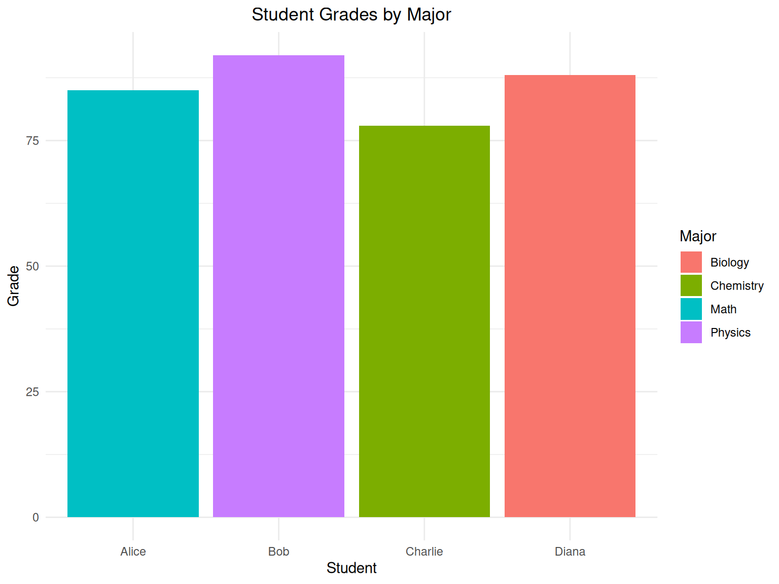

# Save the plot
ggsave(
  plot = p1,
  filename = "figures/student_grades.png",
  width = 8,
  height = 6,
  dpi = 300
)

This chart immediately shows us that Bob has the highest grade (92) and Charlie has the lowest (78). Visualizations like this make patterns in data much easier to spot than looking at numbers alone.

Notice how we:

Store the plot in a variable (p1) before displaying it
Use explicit argument names in ggplot() like data = and mapping =
Save the plot for future use or sharing

3 RStudio: Your R Interface

3.1 What is RStudio?

While you can use R by itself, RStudio (Posit Team 2023) makes the experience much more pleasant and productive. RStudio is an Integrated Development Environment (IDE) that provides a user-friendly interface for R.

3.1.1 The Four-Panel Layout

RStudio organizes your work into four main areas:

Script Editor (top-left): Where you write and edit your R code
- Syntax highlighting makes code easier to read
- Auto-completion helps you write code faster
- You can save your scripts for later use
Console (bottom-left): Where you interact directly with R
- Type commands and see immediate results
- View error messages and warnings
- Test code snippets quickly
Environment/History (top-right): Shows your current workspace
- Environment tab: See all your data objects and variables
- History tab: Review commands you’ve run previously
- Connections tab: Manage database connections
Files/Plots/Packages/Help (bottom-right): Multiple useful tabs
- Files tab: Navigate your computer’s file system
- Plots tab: View charts and graphs you create
- Packages tab: Install and manage R packages
- Help tab: Access documentation and tutorials

3.2 Installing RStudio

RStudio installation is straightforward, but R must be installed first:

Ensure R is installed: RStudio requires R to be installed first
Visit Posit: Go to https://posit.co/downloads/
Choose RStudio Desktop: The free version is perfect for learning
Download and install: Follow the installation wizard with default settings
Launch RStudio: You should see the four-panel interface

3.3 Creating and Managing Projects

One of RStudio’s best features is project management. Projects keep your work organized and make it easy to switch between different analyses:

3.3.1 Why Use Projects?

Organization: Keep related files together
Working Directory: Automatically sets the correct folder
Portability: Easy to share entire projects with others
Version Control: Integrate with Git for tracking changes

3.3.2 Creating Your First Project

# Create directories
dirs <- c("data", "figures", "R", "out")
sapply(dirs, dir.create, showWarnings = FALSE)

# Sample data (data.table already loaded)
sales <-
  data.table(
    month = c("Jan", "Feb", "Mar", "Apr", "May", "Jun"),
    sales = c(100, 120, 150, 130, 160, 180),
    region = rep(c("North", "South"), 3)
  )

# Export files (packages already loaded)
fwrite(x = sales, file = "data/sales.csv")
write.xlsx(x = sales, file = "data/sales.xlsx")

cat("Files created:\n")
list.files(path = "data", full.names = TRUE)

When you create a project, RStudio:

Creates a dedicated folder for your work
Sets up the proper working directory
Remembers your project settings
Makes it easy to share your work with others

Notice how we create an “out” folder to store our output files and saved plots.

4 Introduction to Quarto

4.1 What is Quarto?

Quarto (Allaire et al. 2022) represents the next generation of scientific and technical publishing. It’s a powerful system that allows you to combine code, text, and outputs into professional documents. Think of Quarto as a way to create reports that include:

Your analysis code: So others can see exactly what you did
Results and charts: Automatically generated from your code
Written explanations: Your insights and conclusions
Professional formatting: Ready for sharing or publication

4.1.1 The Power of Reproducible Research

Traditional data analysis often involves:

Analyzing data in one program
Creating charts in another program
Writing conclusions in a word processor
Manually copying results between programs

This approach has problems:

Error-prone: Easy to copy wrong numbers
Time-consuming: Updates require changing multiple files
Not reproducible: Others can’t verify your work

Quarto solves these problems by combining everything in one document that automatically updates when your data or analysis changes.

4.2 Installing Quarto

Quarto installation is simple and integrates seamlessly with RStudio:

Visit the official website: Go to https://quarto.org/docs/get-started/
Download for your system: Choose Windows, macOS, or Linux
Install with defaults: The installer will handle everything
Restart RStudio: This enables Quarto integration
Verify installation: You should see Quarto options in RStudio menus

4.3 Quarto Projects

Quarto projects provide additional organization and publishing features beyond basic RStudio projects:

4.3.1 Creating a Quarto Project

In RStudio:

File → New Project
New Directory
Quarto Project
Choose project type (Document, Website, Book, etc.)
Configure options (output formats, features)
Create Project

4.3.2 Benefits of Quarto Projects

Multiple output formats: HTML, PDF, Word from the same source
Consistent styling: Professional appearance across all outputs
Cross-references: Automatic numbering for figures and tables
Bibliography management: Automatic citation formatting
Website publishing: Easy deployment to GitHub Pages or other platforms

4.4 Your First Document

4.4.1 Creating New Documents

The process is straightforward in RStudio:

File → New File → Quarto Document
Enter document details: Title, author, output format
Choose format: HTML is best for beginners
Click Create: RStudio opens a template document

4.4.2 Understanding Document Structure

Every Quarto document has three main parts:

YAML Header: Configuration between --- lines
Text: Written in Markdown format
Code Chunks: R code between ```{r} and ```

4.4.3 Output Formats

Quarto’s ability to create multiple formats from one source is powerful:

PDF (for printing)

format: pdf

Best for: Professional reports, academic papers
Features: Page numbers, professional typography, print-ready

Word (for collaboration)

format: docx

Best for: Collaborating with non-R users
Features: Compatible with Microsoft Word, easy editing by others

4.5 A Complete Example

Let’s create a complete example that demonstrates Quarto’s capabilities using fastverse functions:

# Weather data
weather <-
  data.table(
    day = c("Mon", "Tue", "Wed", "Thu", "Fri"),
    temp = c(22, 25, 23, 27, 24),
    humidity = c(60, 55, 65, 50, 58),
    condition = c("Sunny", "Cloudy", "Rainy", "Sunny", "Partly Cloudy")
  )

# Statistics with pipe and fastverse
weather %>%
  fsummarise(
    avg_temp = fmean(temp),
    max_temp = fmax(temp),
    min_temp = fmin(temp)
  )

   avg_temp max_temp min_temp
      <num>    <num>    <num>
1:     24.2       27       22

# Create and save visualization
p2 <- ggplot(data = weather, mapping = aes(x = day, y = temp, fill = condition)) +
  geom_col() +
  labs(title = "Daily Temperature", x = "Day", y = "Temperature (°C)", fill = "Condition") +
  theme_minimal() +
  geom_text(mapping = aes(label = paste(temp, "°C")), vjust = -0.3)

# Display the plot
p2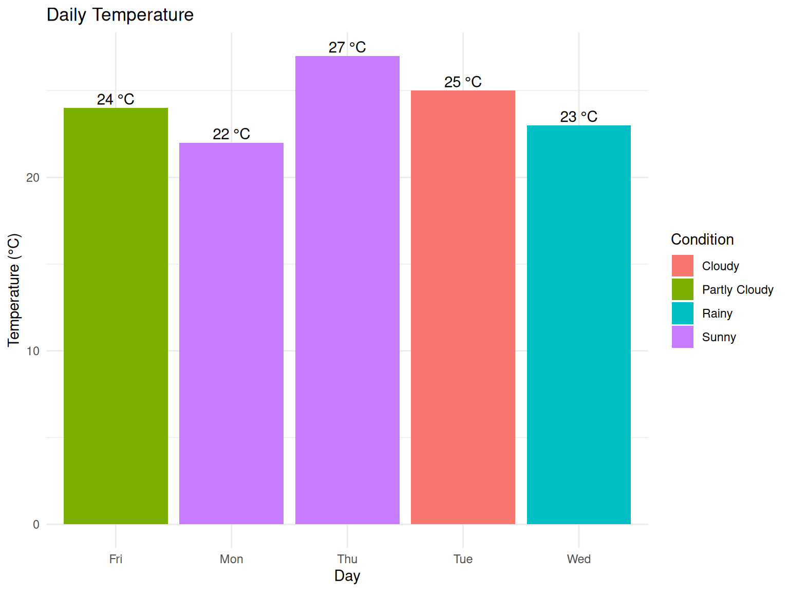

# Save the plot
ggsave(
  plot = p2,
  filename = "figures/daily_temperature.png",
  width = 10,
  height = 6,
  dpi = 300
)

This example demonstrates several key Quarto features:

Code execution: The R code runs automatically
Output capture: Results are included in the document
Figure generation: Charts are created and properly captioned
Professional formatting: Everything looks polished

Notice how we use fmean(), fmax(), and fmin() from fastverse for efficient statistical calculations.

5 Working with Different File Types

5.1 Reading and Writing Data

Modern data analysis often involves working with data stored in various formats. Here’s how to handle the most common ones using efficient functions:

# Read data efficiently with explicit arguments (packages already loaded)
sales_csv <- fread(file = "data/sales.csv")
sales_excel <- read_excel(path = "data/sales.xlsx") %>% as.data.table()

# Compare datasets
identical(x = sales_csv, y = sales_excel)
rbindlist(l = list(CSV = sales_csv, Excel = sales_excel), idcol = "Source")

5.1.1 Understanding File Formats

CSV files: Plain text, widely compatible, smaller file size
Excel files: Can contain multiple sheets, formatted data, larger file size
data.table: More efficient than data.frame for larger datasets

Notice how we use fread() instead of read.csv() - it’s much faster and more flexible.

5.2 Practical Examples

Let’s work through some realistic examples that demonstrate common data analysis tasks using fastverse functions:

# Test scores data
scores <-
  data.table(
    student = c("Anna", "Bob", "Carol", "David", "Eva"),
    math = c(85, 92, 78, 88, 95),
    english = c(88, 85, 92, 80, 90),
    science = c(82, 90, 85, 92, 88)
  )

# Display table with knitr (already loaded)
kable(x = scores, caption = "Student Test Scores")

Student Test Scores
student	math	english	science
Anna	85	88	82
Bob	92	85	90
Carol	78	92	85
David	88	80	92
Eva	95	90	88

# Calculate subject averages using fastverse
subject_summary <-
  scores %>%
  fsummarise(
    Math = fmean(math),
    English = fmean(english),
    Science = fmean(science)
  ) %>%
  pivot(
    how = "longer",
    names = list("Subject", "Average")
  )

kable(x = subject_summary, caption = "Subject Averages", digits = 1)

Subject Averages
Subject	Average
Math	87.6
English	87.0
Science	87.4

This table shows our data in a clean, professional format that’s easy to read and understand.

Now let’s create a comparison visualization:

# Reshape data for visualization
subject_avg <-
  scores %>%
  fsummarise(
    Math    = fmean(math),
    English = fmean(english),
    Science = fmean(science)
  ) %>%
  pivot(
    how = "longer",
    names = list("Subject", "Average")
  )

# Create and save comparison chart
p3 <- ggplot(data = subject_avg, mapping = aes(x = Subject, y = Average, fill = Subject)) +
  geom_col(alpha = 0.8, show.legend = FALSE) +
  labs(title = "Average Test Scores by Subject", x = "Subject", y = "Average Score") +
  theme_minimal() +
  geom_text(mapping = aes(label = round(x = Average, digits = 1)), vjust = -0.3) +
  ylim(0, 100)

# Display the plot
p3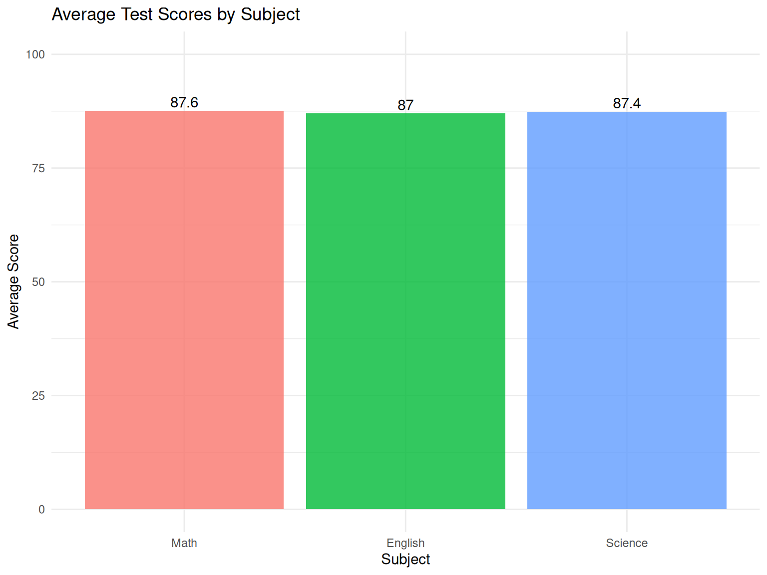

# Save the plot
ggsave(
  plot = p3,
  filename = "figures/subject_averages.png",
  width = 8,
  height = 6,
  dpi = 300
)

This visualization immediately shows that Math scores are slightly higher than English scores on average, demonstrating how charts can reveal patterns that might not be obvious from tables alone.

Notice how we use:

fmean() for calculating averages efficiently
pivot() for reshaping data
Explicit argument names throughout for clarity

6 Essential Tips for Success

6.1 Getting Help When You Need It

Learning R is a journey, and everyone needs help sometimes. Here are the best ways to get assistance:

# Help functions with explicit arguments
?mean
help.search(pattern = "regression")
example(topic = "mean")

# Package help
help(package = "data.table")

6.1.1 Additional Help Resources

RStudio Help pane: Built-in documentation with examples
Stack Overflow: Huge community of R users answering questions
R-bloggers: Daily articles about R techniques and applications
Local R User Groups: Many cities have R meetups and workshops

6.2 Common Mistakes and How to Avoid Them

Learning from common mistakes can save you hours of frustration:

6.2.1 1. Case Sensitivity

R distinguishes between uppercase and lowercase letters:

Mean ≠ mean (only mean is the correct function)
Data ≠ data (variable names must match exactly)

6.2.2 2. Quotation Marks

Text must be enclosed in quotes:

Correct: "Alice", "Sales Department"
Incorrect: Alice, Sales Department

6.2.3 3. Package Loading

Packages must be loaded before use:

Always run library(fastverse) before using fastverse functions
Load packages at the beginning of your script

6.2.4 4. Parentheses and Brackets

Every opening parenthesis needs a closing one:

fmean(students$age) ✓
fmean(students$age ✗ (missing closing parenthesis)

6.2.5 5. Using Explicit Arguments

Always use explicit argument names when learning:

Good: round(x = 3.14159, digits = 2)
Less clear: round(3.14159, 2)

6.3 Keyboard Shortcuts for Efficiency

Learning these shortcuts will significantly speed up your work:

Ctrl+Enter (Windows) or Cmd+Enter (Mac): Run current line or selection
Ctrl+Shift+Enter: Run entire code chunk
Tab: Auto-complete function names and file paths
Ctrl+Z: Undo last action
Ctrl+Shift+C: Comment/uncomment selected lines
Ctrl+L: Clear console
Ctrl+1: Focus on script editor
Ctrl+2: Focus on console

6.4 Best Practices for Beginners

Developing good habits early will save you time and frustration:

6.4.1 1. Project Organization

my-analysis/
├── data/           # Raw data files
├── R/              # R scripts
├── figures/        # Generated plots
├── out/            # Output files
└── README.md       # Project description

6.4.2 2. Code Documentation

# Load required packages
library(data.table)
library(fastverse)
library(ggplot2)

# Read sales data from CSV file
sales_data <- fread(file = "data/sales_2023.csv")

# Calculate monthly averages
monthly_avg <- fmean(x = sales_data$monthly_sales)

6.4.3 3. Consistent Naming

Use descriptive names: student_grades not sg
Be consistent: if you use underscores, always use underscores
Avoid spaces in names: sales_data not sales data

6.4.4 4. Regular Saving

Save your scripts frequently (Ctrl+S)
Use meaningful file names with dates
Consider version control (Git) for important projects

6.4.5 5. Save Your Plots

Always save important visualizations
Use consistent naming for plot files
Store plots in a dedicated folder

7 Troubleshooting Common Issues

7.1 Package-Related Problems

Package issues are among the most common problems beginners encounter:

# If you see "packagename not found"
install.packages("packagename")
library(packagename)

install.packages("ggplot2")
library(ggplot2)

# Install multiple packages
install.packages(c("data.table", "readxl", "openxlsx"))

# Session information
sessionInfo()

7.1.1 Additional Package Solutions

Update R: Newer versions often resolve compatibility issues
Restart R session: Session → Restart R in RStudio
Check internet connection: Package installation requires internet access
Try different mirror: Some CRAN mirrors may be temporarily unavailable

7.2 Data Import Issues

Common problems when loading data:

7.2.1 File Path Problems

Use forward slashes: "data/myfile.csv" not "data\myfile.csv"
Check working directory: Use getwd() to see current location
Use relative paths: Avoid "C:/Users/YourName/Desktop/file.csv"

7.2.2 File Format Issues

Check file extension: Ensure .csv files are actually CSV format
Encoding problems: Try fread(file = "file.csv", encoding = "UTF-8")
Delimiter issues: Some “CSV” files use semicolons or tabs

7.3 Getting More Help

When you’re stuck, try these resources in order:

Built-in Help: Start with ?function_name
RStudio Cheatsheets: Help → Cheatsheets
Google Search: “R how to [your specific question]”
Stack Overflow: Include “R” in your search terms
RStudio Community: community.rstudio.com
Local User Groups: Search for “R User Group [your city]”

8 Conclusion

Congratulations! You’ve completed your introduction to R, RStudio, and Quarto. You now have a solid foundation for data analysis and report creation using modern, efficient tools.

8.1 What You’ve Accomplished

Through this guide, you’ve learned to:

✅ Install and set up the complete R data science toolkit
✅ Perform basic mathematics and statistical calculations with fastverse
✅ Create and manipulate data using data.table()
✅ Generate professional visualizations with ggplot2
✅ Build comprehensive reports with Quarto
✅ Organize projects effectively in RStudio
✅ Troubleshoot common problems independently
✅ Apply best practices for reproducible research
✅ Use explicit arguments for clearer, more readable code

8.2 Your Next Steps

Now that you have the basics, here’s how to continue your learning journey:

Create a personal project: Analyze data you care about (sports, weather, personal finances)
Reproduce this tutorial: Try creating similar analyses with different data
Experiment with styling: Modify colors, themes, and formatting in your charts
Practice explicit arguments: Always use argument names in your functions
Learn more ggplot2: Explore different chart types (scatter plots, histograms, box plots)
Master data import: Practice reading different file formats and cleaning messy data
Develop your workflow: Create templates for common analyses
Explore fastverse: Learn more efficient functions for data manipulation
Statistical methods: Learn about hypothesis testing, regression, and correlation analysis
Advanced Quarto: Explore presentations, websites, and interactive documents
Package ecosystem: Discover specialized packages for your field of interest
Automation: Learn to create functions and automate repetitive tasks

8.3 Essential Learning Resources

8.3.1 Free Online Books

R for Data Science (Wickham and Grolemund 2016): The definitive beginner’s guide
Quarto Documentation: Comprehensive guide to all Quarto features
ggplot2 Book: Deep dive into data visualization
fastverse Documentation: Learn efficient data manipulation

8.3.2 Interactive Learning

RStudio Education: Free courses and tutorials
Swirl: Learn R interactively within R itself
DataCamp: Structured courses (some free content)

8.3.3 Community Resources

R-bloggers: Daily articles and tutorials
#RStats Twitter: Active community sharing tips and resources
Local R Meetups: Network with other R users in your area

8.4 Final Encouragement

Remember that everyone starts as a beginner, and the R community is known for being welcoming and helpful. Don’t be discouraged if concepts take time to sink in—data analysis is a skill that develops with practice.

The tools you’ve learned today are used by:

Data scientists at major technology companies
Researchers at universities worldwide
Analysts in government and non-profit organizations
Students in fields from psychology to finance
Professionals in healthcare, marketing, and countless other fields

You’re now part of a global community of people using these powerful tools to understand the world through data.

Keep practicing, stay curious, and most importantly—have fun with your data analysis journey!

Remember: Always use explicit argument names, save your work regularly, and don’t hesitate to ask for help when you need it.

9 R Packages used

# Load all required packages for this tutorial
library(data.table) # Fast data manipulation and file reading
library(fastverse) # Collection of fast R packages for data science
library(tidyverse) # Collection of packages for data science workflow
library(readxl) # Read Excel files (.xlsx, .xls)
library(openxlsx) # Write Excel files and advanced Excel operations
library(knitr) # Dynamic report generation and table formatting
library(ggplot2) # Advanced data visualization (part of tidyverse)

About the Packages We used

data.table (Dowle and Srinivasan 2023): A high-performance package for working with large datasets. It’s much faster than base R data.frame for reading, writing, and manipulating data.

fastverse: A collection of complementary packages that work together for fast and efficient data science. Includes functions like fmean(), fmax(), etc.

tidyverse (Wickham and Grolemund 2016): A collection of packages designed for data science, including ggplot2 for visualization, dplyr for data manipulation, and readr for data import.

readxl: Specifically designed to read Excel files. It can handle both .xlsx and .xls formats without requiring Excel to be installed.

openxlsx: Allows you to create and write Excel files with formatting, formulas, and multiple sheets.

knitr: Essential for creating dynamic documents. It processes R code chunks and creates formatted tables and reports.

ggplot2: Part of tidyverse, this is the most popular package for creating beautiful, publication-ready visualizations in R.

Happy analyzing!

10 References

Allaire, J. J., Charles Teague, Carlos Scheidegger, Yihui Xie, and Christophe Dervieux. 2022. “Quarto.” GitHub Repository. https://github.com/quarto-dev/quarto-cli.

Dowle, Matt, and Arun Srinivasan. 2023. Data.table: Extension of Data.frame. https://r-datatable.com/.

Posit Team. 2022. “Quarto: An Open-Source Scientific and Technical Publishing System.” https://quarto.org/.

———. 2023. RStudio: Integrated Development Environment for r. Posit Software, PBC. http://www.rstudio.com/.

Wickham, Hadley. 2016. Ggplot2: Elegant Graphics for Data Analysis. Springer-Verlag New York. https://ggplot2.tidyverse.org.

Wickham, Hadley, and Garrett Grolemund. 2016. R for Data Science: Import, Tidy, Transform, Visualize, and Model Data. O’Reilly Media. https://r4ds.had.co.nz/.

1 Introduction

1.1 Why Use These Tools?

2 Getting Started with R

2.1 What is R?

2.2 Installing R

2.3 Basic Math in R

2.4 Working with Data Tables

2.5 Basic Statistics with Fastverse

2.6 Creating and Saving Visualizations

3 RStudio: Your R Interface

3.1 What is RStudio?

3.1.1 The Four-Panel Layout

3.2 Installing RStudio

3.3 Creating and Managing Projects

3.3.1 Why Use Projects?

3.3.2 Creating Your First Project

4 Introduction to Quarto

4.1 What is Quarto?

4.1.1 The Power of Reproducible Research

4.2 Installing Quarto

4.3 Quarto Projects

4.3.1 Creating a Quarto Project

4.3.2 Benefits of Quarto Projects

4.4 Your First Document

4.4.1 Creating New Documents

4.4.2 Understanding Document Structure

4.4.3 Output Formats

HTML (for web sharing)

PDF (for printing)

Word (for collaboration)

4.5 A Complete Example

5 Working with Different File Types

5.1 Reading and Writing Data

5.1.1 Understanding File Formats

5.2 Practical Examples

6 Essential Tips for Success

6.1 Getting Help When You Need It

6.1.1 Additional Help Resources

6.2 Common Mistakes and How to Avoid Them

6.2.1 1. Case Sensitivity

6.2.2 2. Quotation Marks

6.2.3 3. Package Loading

6.2.4 4. Parentheses and Brackets

6.2.5 5. Using Explicit Arguments

6.3 Keyboard Shortcuts for Efficiency

6.4 Best Practices for Beginners

6.4.1 1. Project Organization

6.4.2 2. Code Documentation

6.4.3 3. Consistent Naming

6.4.4 4. Regular Saving

6.4.5 5. Save Your Plots

7 Troubleshooting Common Issues

7.1 Package-Related Problems

7.1.1 Additional Package Solutions

7.2 Data Import Issues

7.2.1 File Path Problems

7.2.2 File Format Issues

7.3 Getting More Help

8 Conclusion

8.1 What You’ve Accomplished

8.2 Your Next Steps

8.3 Essential Learning Resources

8.3.1 Free Online Books

8.3.2 Interactive Learning

8.3.3 Community Resources

8.4 Final Encouragement

9 R Packages used

10 References