knitr::read_chunk("2022-05-20_TUF.R")Statistics: The Art & Science of Learning from Data
Introduction
Statistics
- Statistics is the science of uncertainty & variability
- Statistics turns data into information
- Data -> Information -> Knowledge -> Wisdom
- Data Driven Decisions (3Ds)
- Statistics is the interpretation of Science
- Statistics is the Art & Science of learning from data
Variable
- Characteristic that may vary from individual to individual
- Height, Weight, CGPA etc
Measurement
- Process of assigning numbers or labels to objects or states in accordance with logically accepted rules
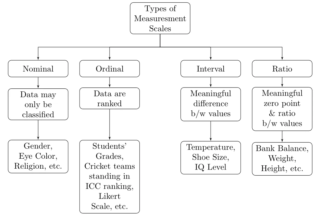
Measurement Scales
- Nominal Scale: Obersvations may be classified into mutually exclusive & exhaustive classes or categories
- Ordinal Scale: Obersvations may be ranked
- Interval Scale: Difference between obersvations is meaningful
- Ratio Scale: Ratio between obersvations is meaningful & true zero point
Exploring Data with Graphs & Numerical Summaries
Graphs
Numerical Summaries
Example
The following data shows the ID, Gender (Male, Female), Age, Race (Mexican American, Non-Hispanic Black, Non-Hispanic White, Other Hispanic, Other/Mixed), BMI, and BMI.Cat (Under Weight, Normal Weight, Over Weight, Obese) from the National Health and Nutrition Examination Survey (NHANES). The survey is conducted by the National Center for Health Statistics (NCHS), and data are publicly available at: https://www.cdc.gov/nchs/nhanes.htm . NHANES data are reported in well over one thousand peer-reviewed journal publications every year.
library(readxl)
library(tidyverse)
Data <-
  read_excel(path = "NHANES1.xlsx") |>
  mutate(
    Gender  = fct_relevel(Gender, "Male", "Female")
  , BMI.Cat = fct_relevel(BMI.Cat, "Under Weight", "Normal Weight", "Over Weight", "Obese")
    )
Data
# A tibble: 8,819 × 6
ID Gender Age Race BMI BMI.Cat
<dbl> <fct> <dbl> <chr> <dbl> <fct>
1 31128 Female 11 Non-Hispanic Black 17.4 Under Weight
2 31129 Male 15 Non-Hispanic Black 26.5 Over Weight
3 31131 Female 44 Non-Hispanic Black 30.9 Obese
4 31132 Male 70 Non-Hispanic White 24.7 Normal Weight
5 31133 Female 16 Non-Hispanic Black 16.8 Under Weight
6 31134 Male 73 Non-Hispanic White 30.6 Obese
7 31137 Female 14 Non-Hispanic Black 27.8 Over Weight
8 31138 Male 3 Mexican American 16.1 Under Weight
9 31139 Female 18 Other Hispanic 29.4 Over Weight
10 31140 Female 11 Non-Hispanic White 18.2 Under Weight
# ℹ 8,809 more rowslibrary(janitor)
Out1 <-
Data |>
tabyl(Gender) |>
adorn_totals(c("row")) |>
adorn_pct_formatting(digits = 2)
Out1 Gender n percent
Male 4305 48.82%
Female 4514 51.18%
Total 8819 100.00%library(scales)
Plot1 <-
ggplot(data = Data, mapping = aes(x = Gender)) +
geom_bar(stat = "count", width = 0.4) +
geom_text(stat = "count", mapping = aes(label = comma(stat(count))), vjust = -0.2) +
scale_y_continuous(
expand = c(0, NA)
, limits = c(0, 4700)
, labels = scales::comma
, breaks = pretty_breaks(12)
) +
labs(
x = "Gender"
, y = "Frequency"
) +
theme_classic() +
theme(aspect.ratio = 2/1)
Plot1Out2 <-
Data |>
tabyl(Gender)
Out2 Gender n percent
Male 4305 0.4881506
Female 4514 0.5118494library(ggchicklet)
Plot2 <-
ggplot(data = Out2, mapping = aes(x = Gender, y = n)) +
geom_chicklet(radius = grid::unit(3, "mm"), width = 0.5) +
geom_text(mapping = aes(label = scales::comma(n)), vjust = -0.2) +
scale_y_continuous(
expand = c(0, NA)
, limits = c(0, 4700)
, labels = scales::comma
, breaks = pretty_breaks(12)
) +
labs(
x = "Gender"
, y = "Frequency"
) +
theme_classic() +
theme(aspect.ratio = 2/1)
Plot2Out3 <-
Data |>
tabyl(Race) |>
adorn_totals(c("row")) |>
adorn_pct_formatting(digits = 2)
Out3 Race n percent
Mexican American 2360 26.76%
Non-Hispanic Black 2392 27.12%
Non-Hispanic White 3350 37.99%
Other Hispanic 291 3.30%
Other/Mixed 426 4.83%
Total 8819 100.00%Plot3 <-
ggplot(data = Data, mapping = aes(x = Race)) +
geom_bar(stat = "count") +
geom_text(stat = "count", mapping = aes(label = comma(stat(count))), vjust = -0.2) +
scale_y_continuous(
expand = c(0, NA)
, limits = c(0, 3500)
, labels = scales::comma
, breaks = pretty_breaks(12)
) +
labs(
x = "Race"
, y = "Frequency"
) +
theme_classic()
Plot3Out4 <-
Data |>
tabyl(BMI.Cat) |>
adorn_totals(c("row")) |>
adorn_pct_formatting(digits = 2)
Out4 BMI.Cat n percent
Under Weight 1921 21.78%
Normal Weight 2770 31.41%
Over Weight 2059 23.35%
Obese 2069 23.46%
Total 8819 100.00%Plot4 <-
ggplot(data = Data, mapping = aes(x = BMI.Cat)) +
geom_bar(stat = "count") +
geom_text(stat = "count", mapping = aes(label = comma(stat(count))), vjust = -0.2) +
scale_y_continuous(
expand = c(0, NA)
, limits = c(0, 3000)
, labels = scales::comma
, breaks = pretty_breaks(12)
) +
labs(
x = "BMI"
, y = "Frequency"
) +
theme_classic()
Plot4Out5 <-
Data |>
tabyl(Gender, BMI.Cat) |>
adorn_totals(c("row", "col")) |>
adorn_percentages("row") |>
adorn_pct_formatting(digits = 2) |>
adorn_ns(position = "front") |>
adorn_title("combined")
Out5 Gender/BMI.Cat Under Weight Normal Weight Over Weight Obese
Male 985 (22.88%) 1,299 (30.17%) 1,115 (25.90%) 906 (21.05%)
Female 936 (20.74%) 1,471 (32.59%) 944 (20.91%) 1,163 (25.76%)
Total 1,921 (21.78%) 2,770 (31.41%) 2,059 (23.35%) 2,069 (23.46%)
Total
4,305 (100.00%)
4,514 (100.00%)
8,819 (100.00%)Plot5 <-
ggplot(data = Data, mapping = aes(x = BMI.Cat, fill = Gender)) +
geom_bar(stat = "count") +
geom_text(stat = "count", mapping = aes(label = comma(stat(count))), vjust = -0.2) +
facet_grid(cols = vars(Gender)) +
scale_y_continuous(
expand = c(0, NA)
, limits = c(0, 1600)
, labels = scales::comma
, breaks = pretty_breaks(12)
) +
labs(
x = "BMI"
, y = "Frequency"
) +
theme_classic()
Plot5Descriptive Statistics
- Number of Observations
- Measures of Central Tendency
- Measures of Central Dispersion
- Measures of Skewness
- Measures of Kurtosis
Example
The following data shows the ID, Gender (Male, Female), Age, Race (Mexican American, Non-Hispanic Black, Non-Hispanic White, Other Hispanic, Other/Mixed), BMI, and BMI.Cat (Under Weight, Normal Weight, Over Weight, Obese) from the National Health and Nutrition Examination Survey (NHANES). The survey is conducted by the National Center for Health Statistics (NCHS), and data are publicly available at: https://www.cdc.gov/nchs/nhanes.htm . NHANES data are reported in well over one thousand peer-reviewed journal publications every year.
Plot6 <-
  ggplot(data = Data, mapping = aes(y = BMI)) +
  geom_boxplot(stat = "boxplot", outlier.colour = "red") +
  scale_x_discrete() +
  scale_y_continuous(
      expand = c(0, NA)
    , limits = c(0, NA)
    , labels = scales::comma
    , breaks = pretty_breaks(12)
    ) +
  labs(
    x = ""
  , y = "BMI"
  ) +
  theme_classic()

Plot6
Plot7 <-
ggplot(data = Data, mapping = aes(y = BMI)) +
geom_boxplot(stat = "boxplot", outlier.colour = "red") +
facet_grid(cols = vars(Gender)) +
scale_x_discrete() +
scale_y_continuous(
expand = c(0, NA)
, limits = c(0, NA)
, labels = scales::comma
, breaks = pretty_breaks(12)
) +
labs(
x = ""
, y = "BMI"
) +
theme_classic()
Plot7library(moments)
Out6 <-
Data |>
summarise(
n = length(BMI)
, Mean = mean(BMI)
, Variance = var(BMI)
, SD = sd(BMI)
, SK = skewness(BMI)
, K = kurtosis(BMI)
)
Out6# A tibble: 1 × 6
n Mean Variance SD SK K
<int> <dbl> <dbl> <dbl> <dbl> <dbl>
1 8819 25.1 57.6 7.59 1.20 8.51Out7 <-
Data |>
filter(BMI < 70) |>
summarise(
n = length(BMI)
, Mean = mean(BMI)
, Variance = var(BMI)
, SD = sd(BMI)
, SK = skewness(BMI)
, K = kurtosis(BMI)
)
Out7# A tibble: 1 × 6
n Mean Variance SD SK K
<int> <dbl> <dbl> <dbl> <dbl> <dbl>
1 8816 25.1 55.8 7.47 0.885 4.19Out8 <-
Data |>
group_by(Gender) |>
summarise(
n = length(BMI)
, Mean = mean(BMI)
, Variance = var(BMI)
, SD = sd(BMI)
, SK = skewness(BMI)
, K = kurtosis(BMI)
)
Out8# A tibble: 2 × 7
Gender n Mean Variance SD SK K
<fct> <int> <dbl> <dbl> <dbl> <dbl> <dbl>
1 Male 4305 24.7 50.9 7.14 1.46 14.8
2 Female 4514 25.4 63.6 7.98 0.994 4.55Out9 <-
Data |>
filter(BMI < 70) |>
group_by(Gender) |>
summarise(
n = length(BMI)
, Mean = mean(BMI)
, Variance = var(BMI)
, SD = sd(BMI)
, SK = skewness(BMI)
, K = kurtosis(BMI)
)
Out9# A tibble: 2 × 7
Gender n Mean Variance SD SK K
<fct> <int> <dbl> <dbl> <dbl> <dbl> <dbl>
1 Male 4304 24.7 48.3 6.95 0.773 4.11
2 Female 4512 25.4 62.6 7.91 0.923 4.07Correlation Analysis
Example
The following data shows the ID, Gender (Male, Female), Age, Race (Mexican American, Non-Hispanic Black, Non-Hispanic White, Other Hispanic, Other/Mixed), BMI, and BMI.Cat (Under Weight, Normal Weight, Over Weight, Obese) from the National Health and Nutrition Examination Survey (NHANES). The survey is conducted by the National Center for Health Statistics (NCHS), and data are publicly available at: https://www.cdc.gov/nchs/nhanes.htm . NHANES data are reported in well over one thousand peer-reviewed journal publications every year.
Out10 <-
  Data |>
  select(BMI, Age) |>
  var()

Out10
BMI Age
BMI 57.55196 81.74215
Age 81.74215 504.62626Out11 <-
Data |>
select(BMI, Age) |>
cor()
Out11 BMI Age
BMI 1.0000000 0.4796573
Age 0.4796573 1.0000000Out12 <-
Data |>
filter(BMI < 70) |>
select(BMI, Age) |>
var()
Out12 BMI Age
BMI 55.76963 81.6055
Age 81.60550 504.7595Out13 <-
Data |>
filter(BMI < 70) |>
select(BMI, Age) |>
cor()
Out13 BMI Age
BMI 1.0000000 0.4863829
Age 0.4863829 1.0000000Data |>
filter(Gender == "Male") |>
select(BMI, Age) |>
var() BMI Age
BMI 50.91307 82.28081
Age 82.28081 531.44024Data |>
filter(Gender == "Male") |>
select(BMI, Age) |>
cor() BMI Age
BMI 1.000000 0.500215
Age 0.500215 1.000000Data |>
filter(Gender == "Female") |>
select(BMI, Age) |>
var() BMI Age
BMI 63.63634 81.5858
Age 81.58580 478.7229Data |>
filter(Gender == "Female") |>
select(BMI, Age) |>
cor() BMI Age
BMI 1.0000000 0.4674336
Age 0.4674336 1.0000000
An Introduction to Linear Models
Regression Analysis
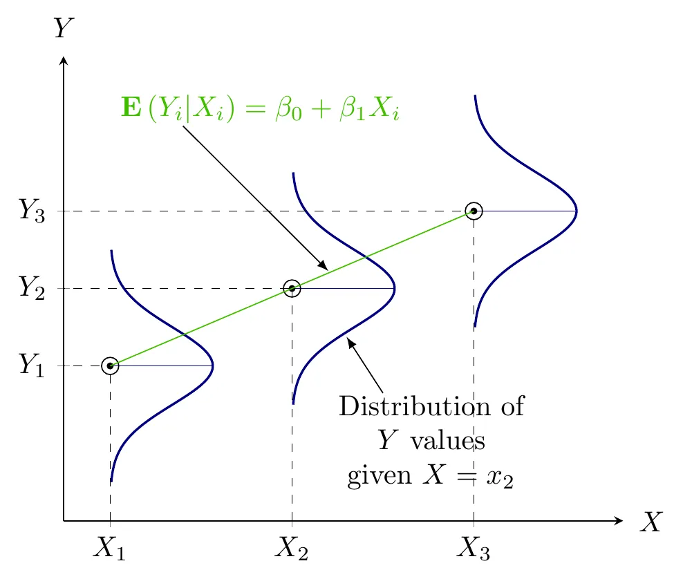
- Quantifying dependency of a normal response on quantitative explanatory variable(s)
Example
The following data shows the ID, Gender (Male, Female), Age, Race (Mexican American, Non-Hispanic Black, Non-Hispanic White, Other Hispanic, Other/Mixed), BMI, and BMI.Cat (Under Weight, Normal Weight, Over Weight, Obese) from the National Health and Nutrition Examination Survey (NHANES). The survey is conducted by the National Center for Health Statistics (NCHS), and data are publicly available at: https://www.cdc.gov/nchs/nhanes.htm . NHANES data are reported in well over one thousand peer-reviewed journal publications every year.
fm1Plot1 <-
  ggplot(data = Data, mapping = aes(x = Age, y = BMI)) +
  geom_point() +
  theme_classic()

fm1Plot1
fm1 <- lm(formula = BMI ~ Age, data = Data)
summary(fm1)$coef Estimate Std. Error t value Pr(>|t|)
(Intercept) 20.3072818 0.116956424 173.6312 0
Age 0.1619855 0.003155804 51.3294 0anova(fm1)Analysis of Variance Table
Response: BMI
Df Sum Sq Mean Sq F value Pr(>F)
Age 1 116760 116760 2634.7 < 2.2e-16 ***
Residuals 8817 390734 44
---
Signif. codes: 0 '***' 0.001 '**' 0.01 '*' 0.05 '.' 0.1 ' ' 1library(emmeans)
fm1Plot2 <-
emmip(
object = fm1
, formula = ~ Age
, cov.reduce = range
) +
scale_x_continuous(breaks = pretty_breaks(12)) +
scale_y_continuous(breaks = pretty_breaks(12)) +
labs(x = "Age", y = "BMI") +
theme_classic()
fm1Plot2library(ggpmisc)
fm1Plot3 <-
ggplot(data = Data, mapping = aes(x = Age, y = BMI)) +
geom_point() +
geom_smooth(method = "lm", se = FALSE, color = "black", formula = y ~ x) +
stat_poly_eq(
formula = y ~ x
, eq.with.lhs = FALSE
, mapping = aes(
label = paste("widehat(italic(BMI))", "~`=`~", gsub("italic(x)","Age",..eq.label..,fixed = TRUE), "~~~", ..rr.label.., "~~~", ..adj.rr.label.., "~~~", ..p.value.label.. , sep = "")
)
, size = 4.5
, parse = TRUE
) +
theme_classic()
fm1Plot3Analysis of Variance (ANOVA)
- Comparing means of Normal dependent variable for levels of different factor(s)
Example
The following data shows the ID, Gender (Male, Female), Age, Race (Mexican American, Non-Hispanic Black, Non-Hispanic White, Other Hispanic, Other/Mixed), BMI, and BMI.Cat (Under Weight, Normal Weight, Over Weight, Obese) from the National Health and Nutrition Examination Survey (NHANES). The survey is conducted by the National Center for Health Statistics (NCHS), and data are publicly available at: https://www.cdc.gov/nchs/nhanes.htm . NHANES data are reported in well over one thousand peer-reviewed journal publications every year.
fm2 <- lm(formula = BMI ~ Gender, data = Data)
anova(fm2)
Analysis of Variance Table
Response: BMI
Df Sum Sq Mean Sq F value Pr(>F)
Gender 1 1173 1172.53 20.418 6.304e-06 ***
Residuals 8817 506321 57.43
---
Signif. codes: 0 '***' 0.001 '**' 0.01 '*' 0.05 '.' 0.1 ' ' 1Analysis of Covariance (ANCOVA)
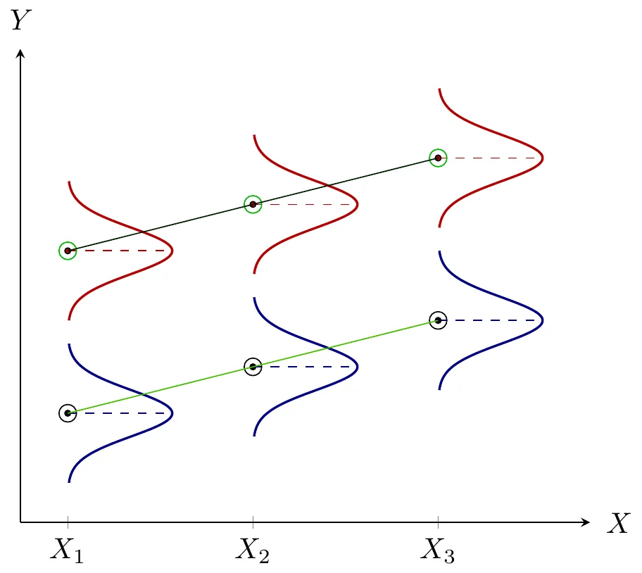
- Quantifying dependency of a normal response on quantitative explanatory variable(s)
- Comparing means of Normal dependent variable for levels of different factor(s)
Example
The following data shows the ID, Gender (Male, Female), Age, Race (Mexican American, Non-Hispanic Black, Non-Hispanic White, Other Hispanic, Other/Mixed), BMI, and BMI.Cat (Under Weight, Normal Weight, Over Weight, Obese) from the National Health and Nutrition Examination Survey (NHANES). The survey is conducted by the National Center for Health Statistics (NCHS), and data are publicly available at: https://www.cdc.gov/nchs/nhanes.htm . NHANES data are reported in well over one thousand peer-reviewed journal publications every year.
fm3 <- lm(formula = BMI ~ Age*Gender, data = Data)
anova(fm3)
Analysis of Variance Table
Response: BMI
Df Sum Sq Mean Sq F value Pr(>F)
Age 1 116760 116760 2647.6079 < 2.2e-16 ***
Gender 1 1722 1722 39.0430 4.338e-10 ***
Age:Gender 1 270 270 6.1294 0.01331 *
Residuals 8815 388742 44
---
Signif. codes: 0 '***' 0.001 '**' 0.01 '*' 0.05 '.' 0.1 ' ' 1summary(fm3)$coef Estimate Std. Error t value Pr(>|t|)
(Intercept) 20.06946217 0.165999451 120.900775 0.000000e+00
Age 0.15482609 0.004390925 35.260475 6.652534e-255
GenderFemale 0.42441011 0.233467368 1.817856 6.912004e-02
Age:GenderFemale 0.01559778 0.006300190 2.475763 1.331382e-02


