Data Analysis with R: Introduction of R Language

Statistics

Research

Author

Muhammad Arfan Dilber

Published

March 25, 2018

The Workspace

The workspace is your current R working environment and includes any user-defined objects (vectors, matrices, data frames, lists, functions). At the end of an R session, the user can save an image of the current workspace that is automatically reloaded the next time R is started.

getwd()

[1] "/media/myaseen208/Documents1/MYaseen208/Consultancy/Mr._M._Yaseen/01Website/myaseen208/blogs/2018-03-25_Maldives_R"

#setwd("C:/Users/PBS FAISALABAD/Documents/R/Training")#use forward slash instead of back slash in windows.
save.image() # To save workspace image.
x<-c(1:4)
x

[1] 1 2 3 4

save(x, file = "mydat.RData")
rm(list = ls())
load("mydat.RData")
x

[1] 1 2 3 4

Data types

x<-2.56
class(x)

[1] "numeric"

[1] 2.56

y<-as.integer(x)
class(y)

[1] "integer"

[1] 2

z<-as.integer(2.56)
z

[1] 2

is.integer(z)

[1] TRUE

as.integer(is.integer(z))

[1] 1

as.integer(!is.integer(z))

[1] 0

as.integer(is.integer(x))

[1] 0

x<-round(x,digits = 1)
x

[1] 2.6

y<-"Male"
class(y)

[1] "character"

Vectors

A vector is a sequence of data elements of the same basic type. A combine function c() is used to form the vector. Here are examples of each type of vector:

x<-c(1,2,3,4)
x

[1] 1 2 3 4

y<-c("a","b","c","d")
y

[1] "a" "b" "c" "d"

c(x,y)

[1] "1" "2" "3" "4" "a" "b" "c" "d"

length(y)

[1] 4

y[c(2,4)]

[1] "b" "d"

y[c(2:4)]

[1] "b" "c" "d"

y[-3]

[1] "a" "b" "d"

names(x)<-c("first","second","third","fourth")
x

 first second  third fourth 
     1      2      3      4

x[c("second","fourth")]

second fourth 
     2      4

x[2]<-5
x

 first second  third fourth 
     1      5      3      4

x<-x*2
x

 first second  third fourth 
     2     10      6      8

seq(from = 1, to = 10, by = 2)

[1] 1 3 5 7 9

rep(5, time = 10)

 [1] 5 5 5 5 5 5 5 5 5 5

rep(c("Male","Female"),time = 10)

 [1] "Male"   "Female" "Male"   "Female" "Male"   "Female" "Male"   "Female"
 [9] "Male"   "Female" "Male"   "Female" "Male"   "Female" "Male"   "Female"
[17] "Male"   "Female" "Male"   "Female"

rep(c("Male","Female"), each = 10)

 [1] "Male"   "Male"   "Male"   "Male"   "Male"   "Male"   "Male"   "Male"  
 [9] "Male"   "Male"   "Female" "Female" "Female" "Female" "Female" "Female"
[17] "Female" "Female" "Female" "Female"

rep(seq(from = 2, to = 9, by = .25), time = 5)

  [1] 2.00 2.25 2.50 2.75 3.00 3.25 3.50 3.75 4.00 4.25 4.50 4.75 5.00 5.25 5.50
 [16] 5.75 6.00 6.25 6.50 6.75 7.00 7.25 7.50 7.75 8.00 8.25 8.50 8.75 9.00 2.00
 [31] 2.25 2.50 2.75 3.00 3.25 3.50 3.75 4.00 4.25 4.50 4.75 5.00 5.25 5.50 5.75
 [46] 6.00 6.25 6.50 6.75 7.00 7.25 7.50 7.75 8.00 8.25 8.50 8.75 9.00 2.00 2.25
 [61] 2.50 2.75 3.00 3.25 3.50 3.75 4.00 4.25 4.50 4.75 5.00 5.25 5.50 5.75 6.00
 [76] 6.25 6.50 6.75 7.00 7.25 7.50 7.75 8.00 8.25 8.50 8.75 9.00 2.00 2.25 2.50
 [91] 2.75 3.00 3.25 3.50 3.75 4.00 4.25 4.50 4.75 5.00 5.25 5.50 5.75 6.00 6.25
[106] 6.50 6.75 7.00 7.25 7.50 7.75 8.00 8.25 8.50 8.75 9.00 2.00 2.25 2.50 2.75
[121] 3.00 3.25 3.50 3.75 4.00 4.25 4.50 4.75 5.00 5.25 5.50 5.75 6.00 6.25 6.50
[136] 6.75 7.00 7.25 7.50 7.75 8.00 8.25 8.50 8.75 9.00

Matrices

A matrix is a collection of data elements arranged in a two dimensional rectangular layout. Matrices are created with the matrix function.

A <- matrix(
  c(1,2,3,4),
  nrow = 2,
  ncol = 2,
  byrow = TRUE)
B <- matrix(
  c(1,2,3,4,5,6,7,8,9),
  nrow = 3,
  ncol = 3,
  byrow = FALSE)
B

     [,1] [,2] [,3]
[1,]    1    4    7
[2,]    2    5    8
[3,]    3    6    9

     [,1] [,2]
[1,]    1    2
[2,]    3    4

A[2,]

[1] 3 4

A[,2]

[1] 2 4

A[2,2]

[1] 4

t(A)

     [,1] [,2]
[1,]    1    3
[2,]    2    4

det(A)

[1] -2

diag(A)

[1] 1 4

B<-A + A
B

     [,1] [,2]
[1,]    2    4
[2,]    6    8

Asquared<- A %*% A
Asquared

     [,1] [,2]
[1,]    7   10
[2,]   15   22

Ainv<- solve(A)
Ainv

     [,1] [,2]
[1,] -2.0  1.0
[2,]  1.5 -0.5

Aev<- eigen(A)
Aev

eigen() decomposition
$values
[1]  5.3722813 -0.3722813

$vectors
           [,1]       [,2]
[1,] -0.4159736 -0.8245648
[2,] -0.9093767  0.5657675

Aev$values

[1]  5.3722813 -0.3722813

Aev$vectors

           [,1]       [,2]
[1,] -0.4159736 -0.8245648
[2,] -0.9093767  0.5657675

Lists

Lists are the most complex of the R data types. Basically, a list is an ordered collection of objects (components). A list allows you to gather a variety of (possibly unrelated) objects under one name. For example, a list may contain a combination of vectors, matrices, data frames, and even other lists. A list is created with the list() function.

g<-"My First List"
h<-c(25,26,18,39)
j<-matrix(1:10, nrow = 5)
k<-c("one", "two", "three")
mylist<-list(title = g, ages = h, j,k)
mylist

$title
[1] "My First List"

$ages
[1] 25 26 18 39

[[3]]
     [,1] [,2]
[1,]    1    6
[2,]    2    7
[3,]    3    8
[4,]    4    9
[5,]    5   10

[[4]]
[1] "one"   "two"   "three"

Data Frames

A Data Frame is used for storing data tables. It is a list of vectors of equal length. Different columns can contain different type of data (numeric,character, etc.). A data frame is created with the data.frame() function:

df<-data.frame(x,y)
df

        x y
first   2 a
second 10 b
third   6 c
fourth  8 d

nrow(df)

[1] 4

ncol(df)

[1] 2

df1<-df[df$y %in% c("a","d"),]
df1

       x y
first  2 a
fourth 8 d

df1<-df[df[,2] %in% c("b","c"),]
df1

        x y
second 10 b
third   6 c

library(PakPC2017)
data(PakPC2017Tehsil)
head(PakPC2017Tehsil)

# A tibble: 6 × 6
  Province Division   District   Tehsil            Pop1998 Pop2017
  <chr>    <chr>      <chr>      <chr>               <dbl>   <dbl>
1 Punjab   Bahawalpur Bahawalpur Hasilpur           317513  456006
2 Punjab   Bahawalpur Bahawalpur Khairpur Tamewali  183903  262628
3 Punjab   Bahawalpur Bahawalpur Yazman             168950  262175
4 Punjab   Bahawalpur Bahawalpur Ahmadpur East      718297 1078683
5 Punjab   Bahawalpur Bahawalpur Bahawalpur City    419542  681696
6 Punjab   Bahawalpur Bahawalpur Bahawalpur Saddar  387038  574950

Reading/writing data from/to files (Import/Export Data)

library(readxl)
spi <- read_excel("C:/Users/PBS FAISALABAD/Desktop/spi.xls")
DT::datatable(spi,fillContainer = TRUE, editable = TRUE)
write.csv(PakPC2017Tehsil,"Population.csv")

Connecting to the database

library(dplyr)
con <- DBI::dbConnect(odbc::odbc(),
                      dsn = "mydata")
table13<-tbl(con, "RPI")
table13
#tehsil<-PakPC2017::PakPC2017Tehsil
#copy_to(con,tehsil,"tehsil",
#        temporary = FALSE
#      )
DBI::dbDisconnect(con)

Numerical or Graphical Summaries of data.

library(PakPC2017)
summary(PakPC2017Tehsil)

   Province           Division           District            Tehsil         
 Length:543         Length:543         Length:543         Length:543        
 Class :character   Class :character   Class :character   Class :character  
 Mode  :character   Mode  :character   Mode  :character   Mode  :character  
                                                                            
                                                                            
                                                                            
                                                                            
    Pop1998           Pop2017       
 Min.   :   3024   Min.   :   2665  
 1st Qu.:  57502   1st Qu.:  89801  
 Median : 157142   Median : 254647  
 Mean   : 240553   Mean   : 377084  
 3rd Qu.: 298074   3rd Qu.: 447854  
 Max.   :2219399   Max.   :4269079  
                   NA's   :1

pairs(PakPC2017Tehsil[,5:6])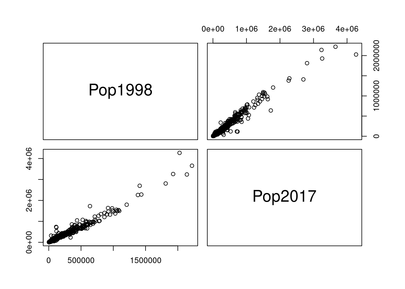

cor(PakPC2017Tehsil[,5:6], use = "complete")

          Pop1998   Pop2017
Pop1998 1.0000000 0.9788354
Pop2017 0.9788354 1.0000000

popLm<-lm(formula = Pop2017 ~ Pop1998, data = PakPC2017Tehsil)
popLm


Call:
lm(formula = Pop2017 ~ Pop1998, data = PakPC2017Tehsil)

Coefficients:
(Intercept)      Pop1998  
  -3445.895        1.579

head(resid(popLm),10)

         1          2          3          4          5          6          7 
-42044.030 -24391.708  -1227.192 -52385.341  22496.260 -32911.295 -36767.021 
         8          9         10 
-92325.684 -73938.014  10353.258

head(fitted(popLm),10)

        1         2         3         4         5         6         7         8 
 498050.0  287019.7  263402.2 1131068.3  659199.7  607861.3  851910.0  783546.7 
        9        10 
 599536.0  143090.7

summary(popLm)


Call:
lm(formula = Pop2017 ~ Pop1998, data = PakPC2017Tehsil)

Residuals:
    Min      1Q  Median      3Q     Max 
-299426  -29128    -355   18117 1071215 

Coefficients:
              Estimate Std. Error t value Pr(>|t|)    
(Intercept) -3.446e+03  5.391e+03  -0.639    0.523    
Pop1998      1.579e+00  1.421e-02 111.147   <2e-16 ***
---
Signif. codes:  0 '***' 0.001 '**' 0.01 '*' 0.05 '.' 0.1 ' ' 1

Residual standard error: 96960 on 540 degrees of freedom
  (1 observation deleted due to missingness)
Multiple R-squared:  0.9581,    Adjusted R-squared:  0.958 
F-statistic: 1.235e+04 on 1 and 540 DF,  p-value: < 2.2e-16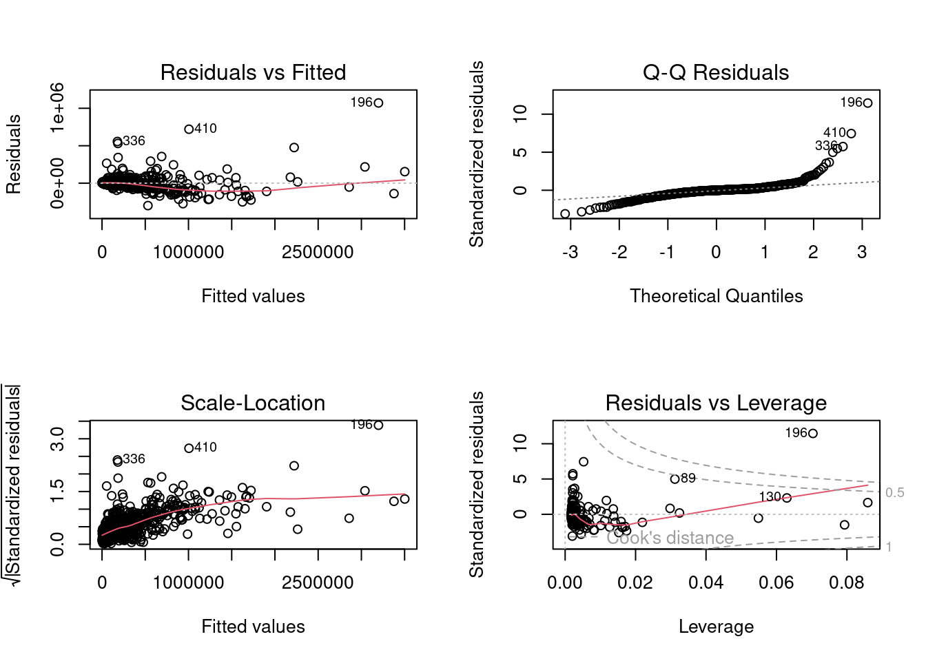

par(mfrow = c(2,2))
plot(popLm)

Summarize Data

library(PakPC2017)
library(dplyr)

Bar charts and Dot charts

library(PakPC2017)
data("PakPC2017Tehsil")
head(PakPC2017Tehsil)

# A tibble: 6 × 6
  Province Division   District   Tehsil            Pop1998 Pop2017
  <chr>    <chr>      <chr>      <chr>               <dbl>   <dbl>
1 Punjab   Bahawalpur Bahawalpur Hasilpur           317513  456006
2 Punjab   Bahawalpur Bahawalpur Khairpur Tamewali  183903  262628
3 Punjab   Bahawalpur Bahawalpur Yazman             168950  262175
4 Punjab   Bahawalpur Bahawalpur Ahmadpur East      718297 1078683
5 Punjab   Bahawalpur Bahawalpur Bahawalpur City    419542  681696
6 Punjab   Bahawalpur Bahawalpur Bahawalpur Saddar  387038  574950

province<-tapply(PakPC2017Tehsil$Pop2017,PakPC2017Tehsil$Province,sum,na.rm=TRUE)
par(mfrow = c(3,2))
dotchart(province)
barplot(province)
boxplot(Pop2017~Province,data = PakPC2017Tehsil)
pie(province, col = rainbow(length(province)))
plot(province, type = "o")
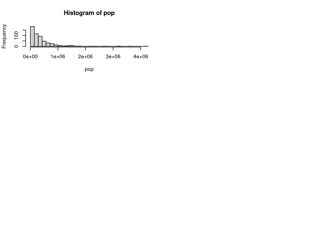
pop<-PakPC2017Tehsil$Pop2017
hist(pop)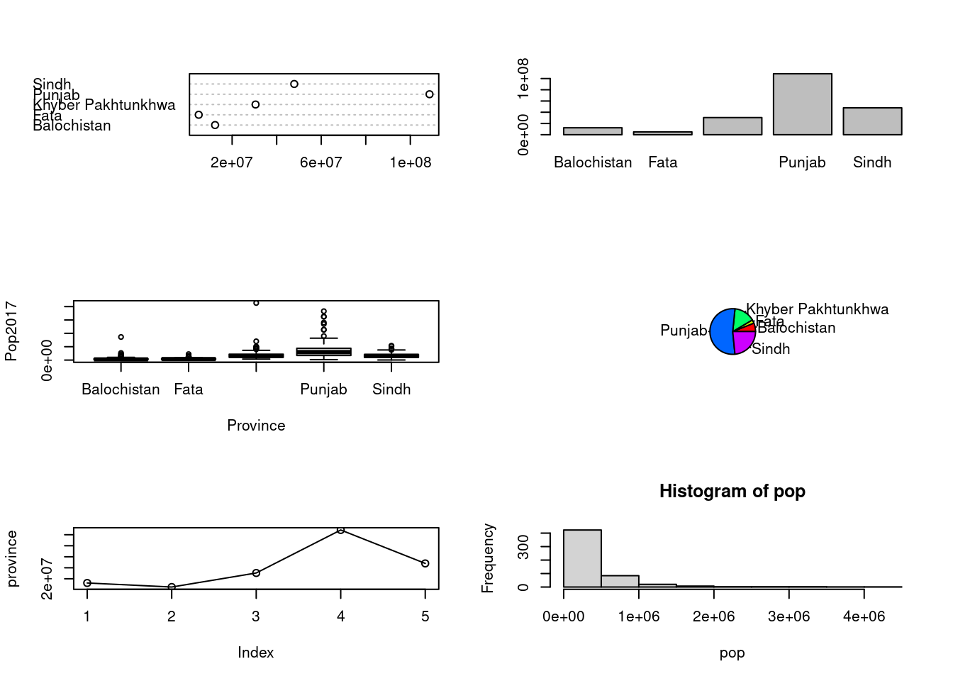

hist(pop, breaks = seq(min(pop,na.rm = TRUE),max(pop,na.rm = TRUE), length.out = 31))

ggplot2 package

The mpg Data Frame

A data frame is a rectangular collection of variables (in the columns) and observations (in the rows). mpg contains observations collected by the US Environment Protection Agency on 38 models of cars; To learn more about mpg, open its help page by running ?mpg.

library(ggplot2)
ggplot(data = mpg)+
  geom_point(mapping = aes(x = displ, y = hwy))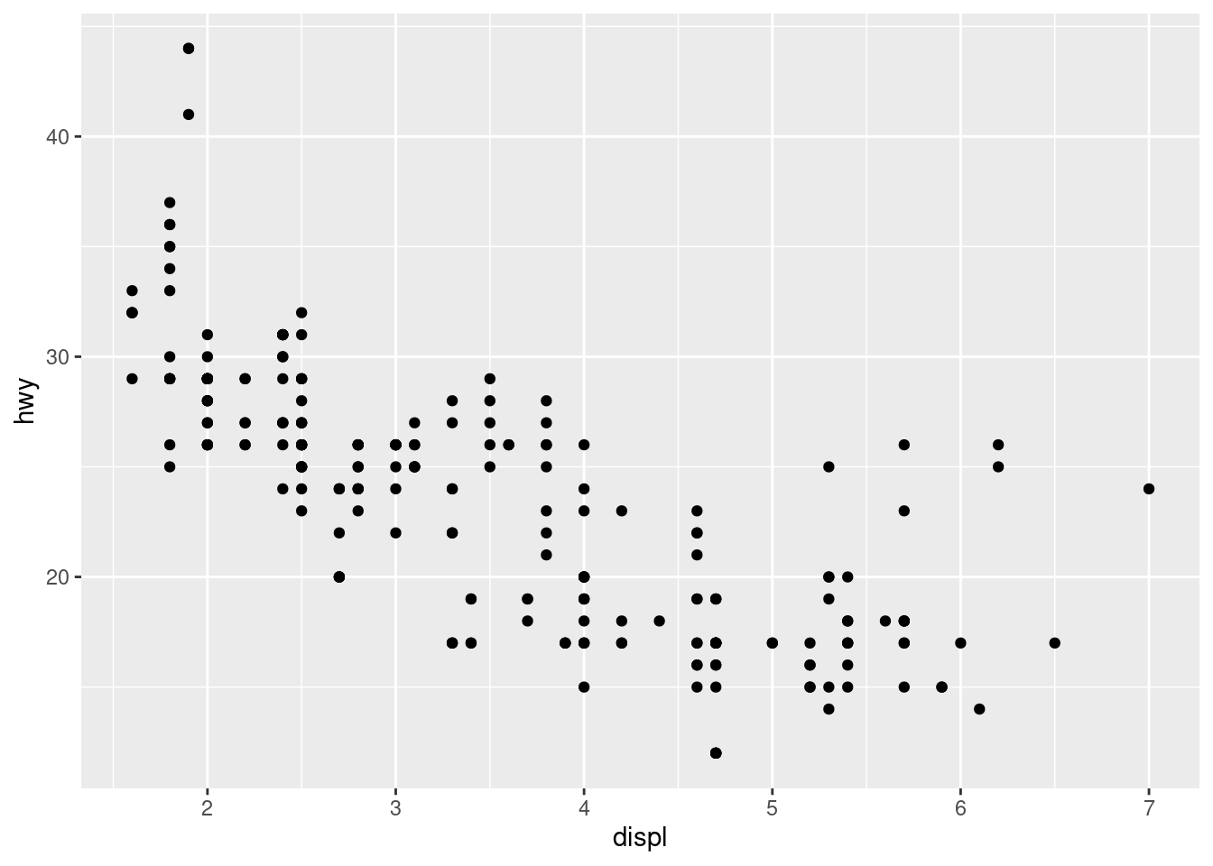

ggplot(data = mpg)+
  geom_point(mapping = aes(x = displ, y = hwy, color = class))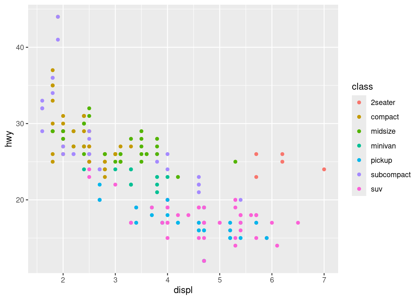

ggplot(data = mpg)+
  geom_point(mapping = aes(x = displ, y = hwy, size = class))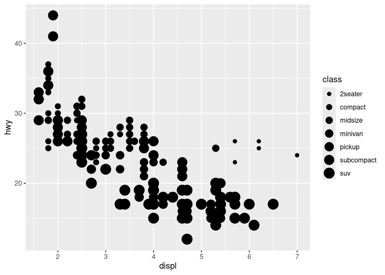

ggplot(data = mpg)+
  geom_point(mapping = aes(x = displ, y = hwy, shape = class))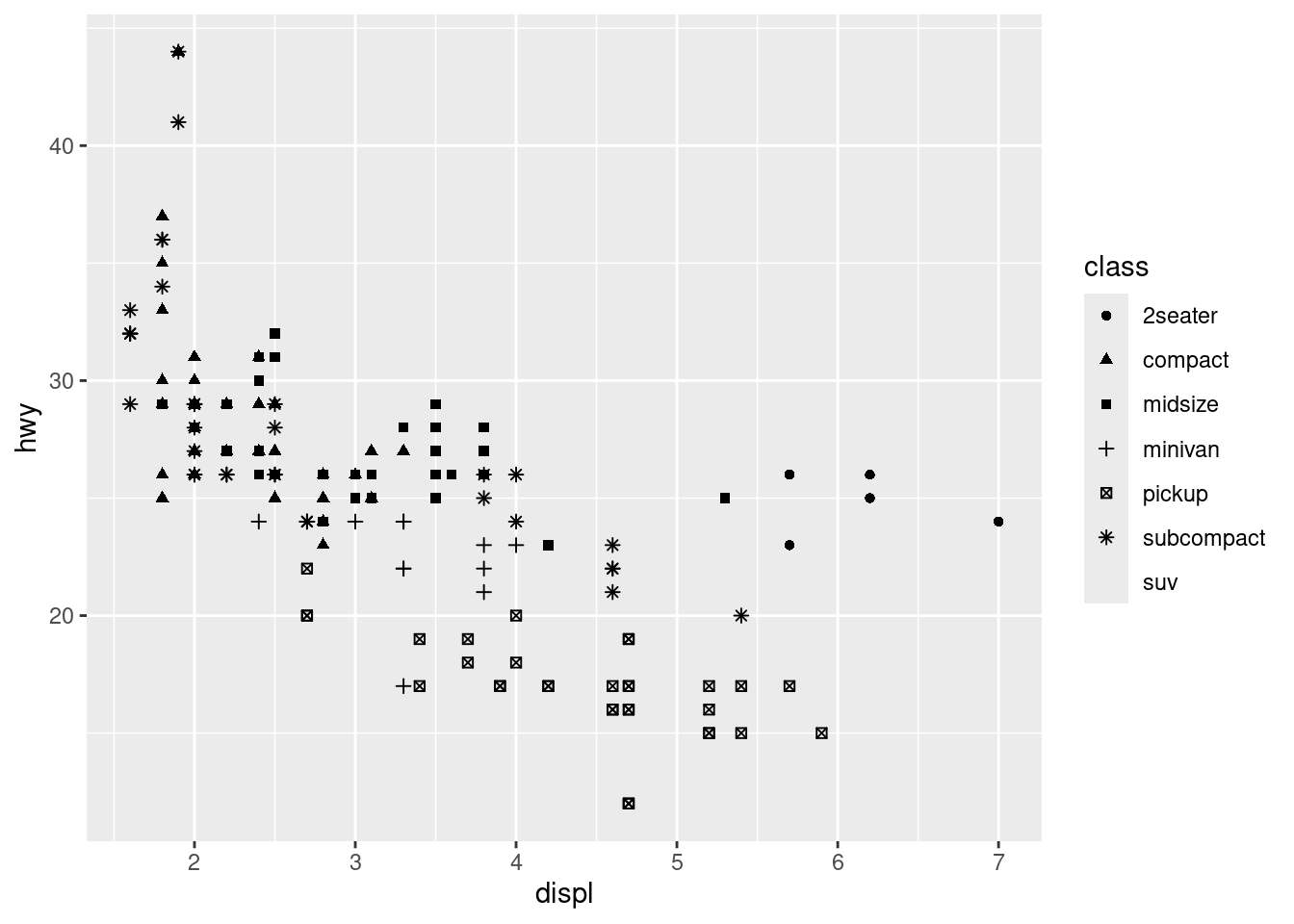

ggplot(data = mpg)+
  geom_point(mapping = aes(x = displ, y = hwy), color = "blue")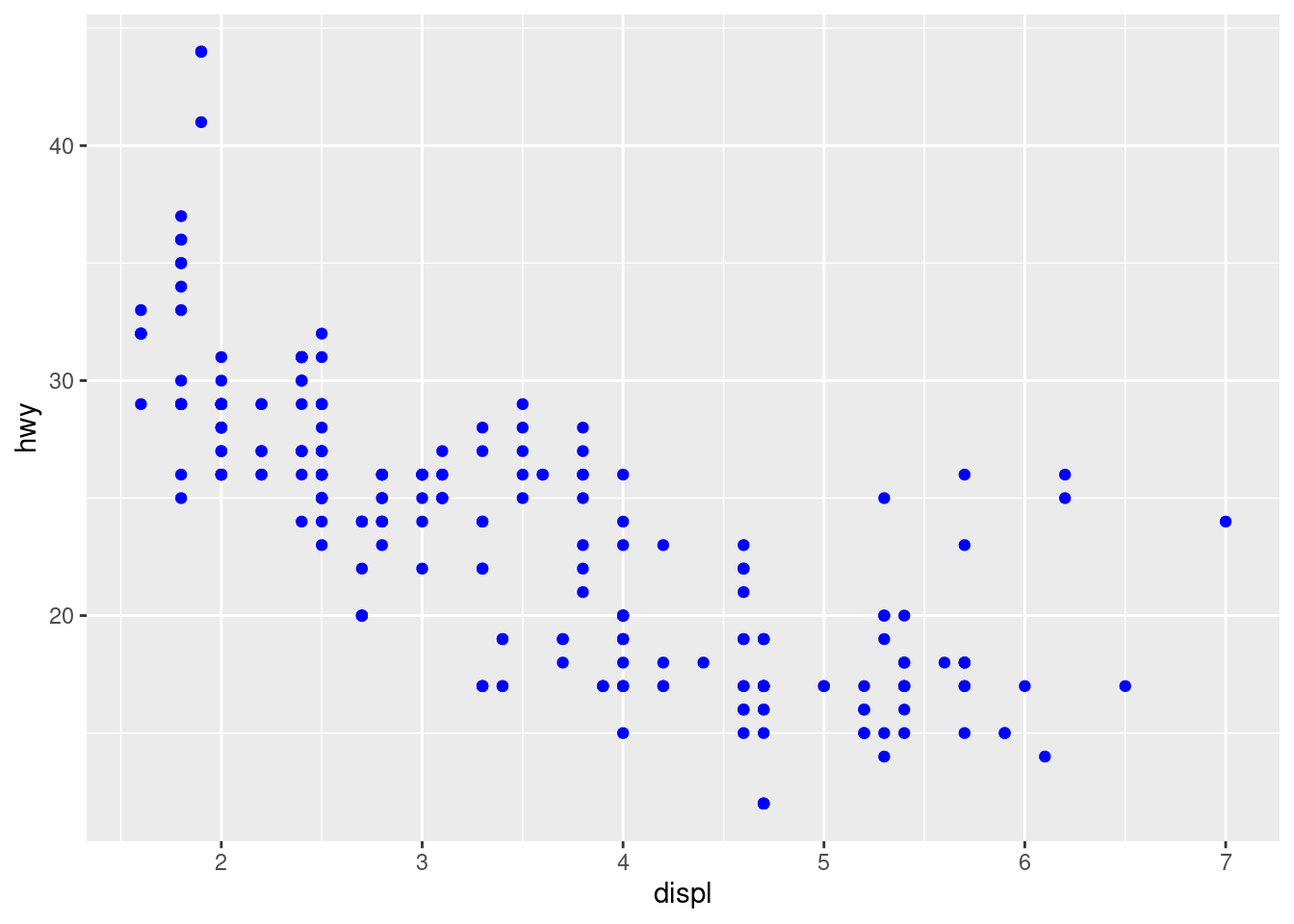

ggplot(data = mpg)+
  geom_smooth(mapping = aes(x = displ, y = hwy))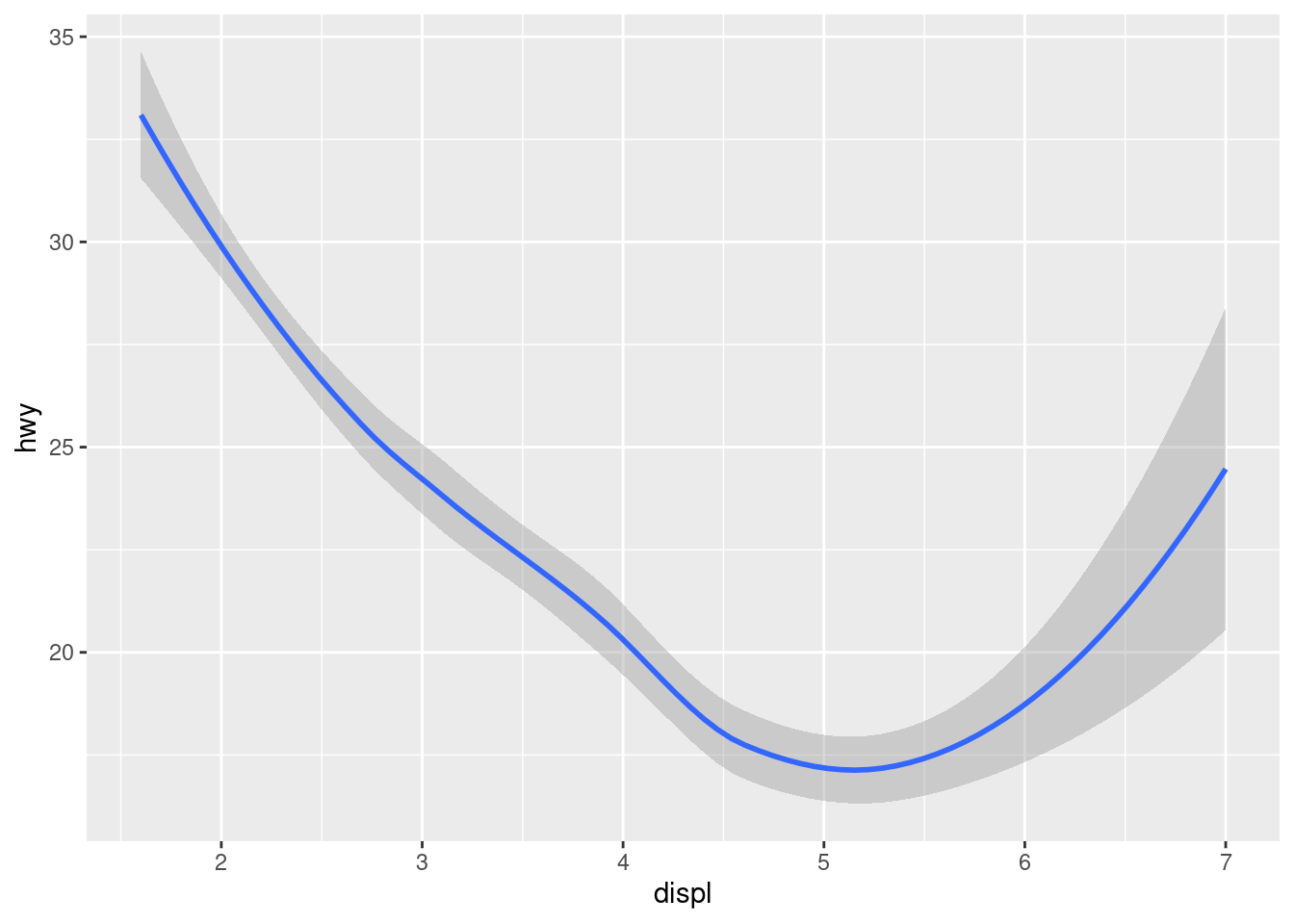

ggplot(data = mpg)+
  geom_smooth(mapping = aes(x = displ, y = hwy, linetype = drv))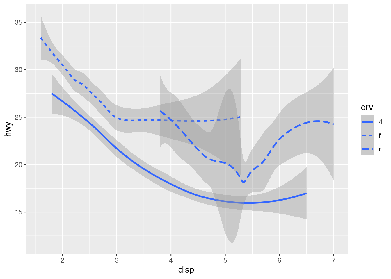

ggplot(data = mpg)+
  geom_point(mapping = aes(x = displ, y = hwy, color = drv))+
  geom_smooth(mapping = aes(x = displ, y = hwy, linetype = drv))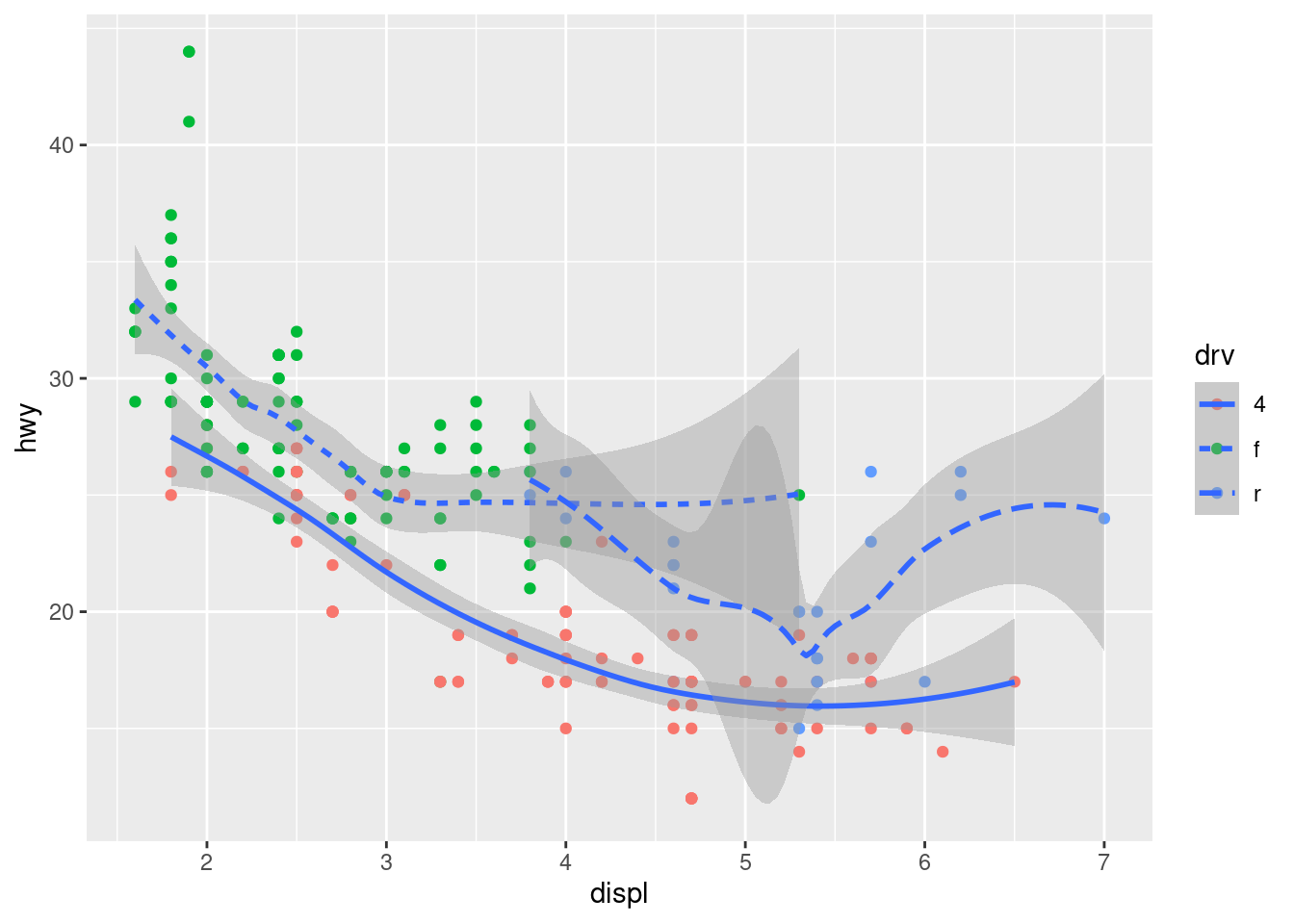

ggplot(data = mpg, mapping = aes(x = displ, y = hwy, color = drv))+
  geom_point()+
  geom_smooth()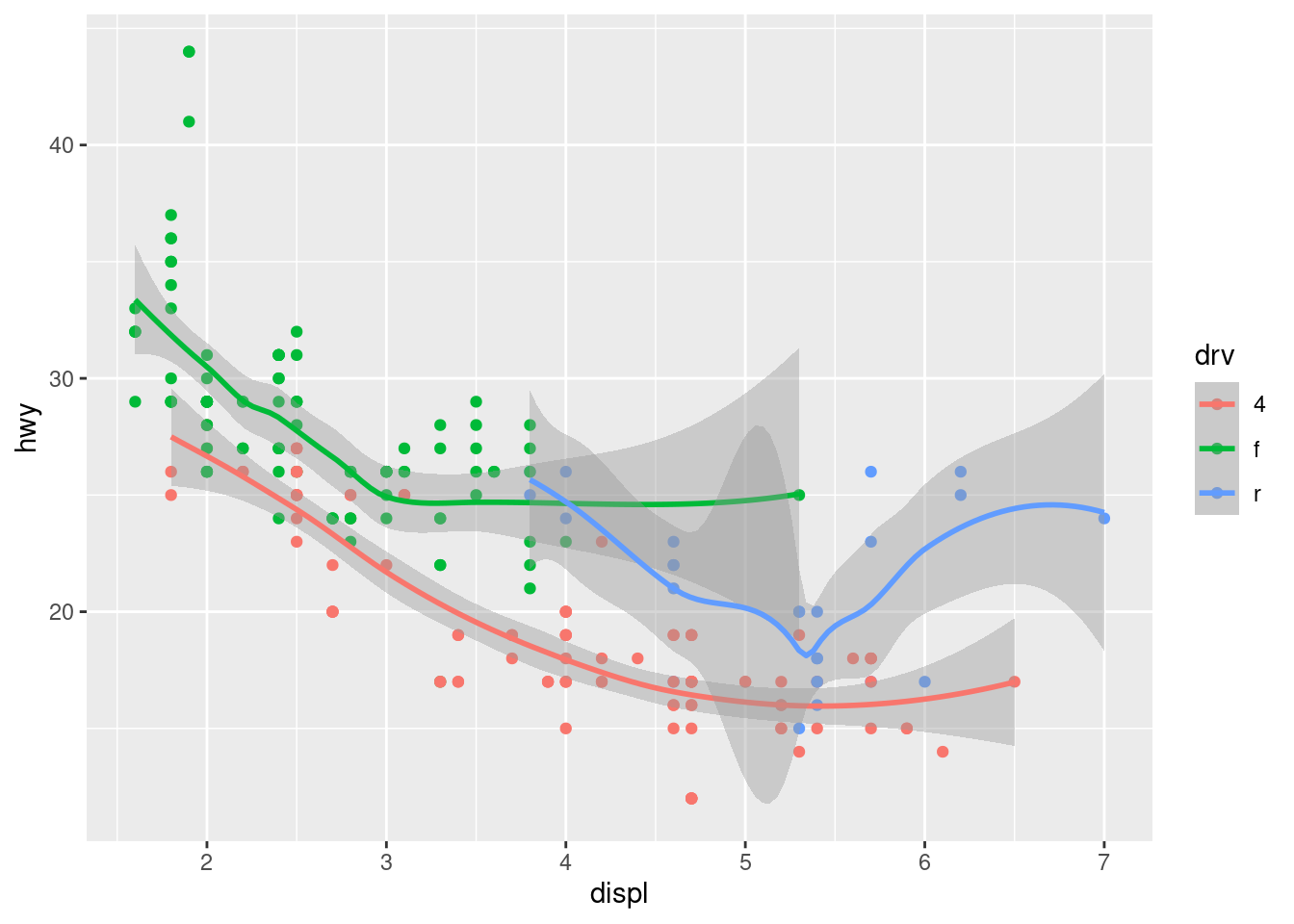

ggplot(data = mpg, mapping = aes(x = displ, y = hwy))+
  geom_point(mapping = aes(color = drv))+
  geom_smooth(mapping = aes(linetype = drv))

Data Transformation

To explore the basic data manipulation we’ll use PakPC2017::PakPC2017Tehsil. This data frame contains the popualtion of all 543 tehsils of Pakistan. The data comes from Pakistan Bureau of Statistics, Population Census 2017, and is documented in ?PakPc2017Tehsil.

library(PakPC2017)
library(dplyr)
tehsil<-as_tibble(PakPC2017Tehsil)
tehsil

# A tibble: 543 × 6
   Province Division   District     Tehsil            Pop1998 Pop2017
   <chr>    <chr>      <chr>        <chr>               <dbl>   <dbl>
 1 Punjab   Bahawalpur Bahawalpur   Hasilpur           317513  456006
 2 Punjab   Bahawalpur Bahawalpur   Khairpur Tamewali  183903  262628
 3 Punjab   Bahawalpur Bahawalpur   Yazman             168950  262175
 4 Punjab   Bahawalpur Bahawalpur   Ahmadpur East      718297 1078683
 5 Punjab   Bahawalpur Bahawalpur   Bahawalpur City    419542  681696
 6 Punjab   Bahawalpur Bahawalpur   Bahawalpur Saddar  387038  574950
 7 Punjab   Bahawalpur Bahawalnagar Bahawalnagar       541553  815143
 8 Punjab   Bahawalpur Bahawalnagar Chishtian          498270  691221
 9 Punjab   Bahawalpur Bahawalnagar Haroonabad         381767  525598
10 Punjab   Bahawalpur Bahawalnagar Fort Abbas          92777  153444
# ℹ 533 more rows

Filter Rows with filter()

filter() allows you to subset observations based on their vaues. The first argument is the name of the data frame. The second and subsequent arguments are the expressions that filter the data frame. For example, we can select all tehsils of Division Faisalabad:

filter(tehsil, Division == "Faisalabad")

# A tibble: 17 × 6
   Province Division   District       Tehsil            Pop1998 Pop2017
   <chr>    <chr>      <chr>          <chr>               <dbl>   <dbl>
 1 Punjab   Faisalabad Faisalabad     Faisalabad City   2140346 3237961
 2 Punjab   Faisalabad Faisalabad     Faisalabad Saddar  924110 1465411
 3 Punjab   Faisalabad Faisalabad     Chak Jhumra        253806  332461
 4 Punjab   Faisalabad Faisalabad     Sammundri          508637  643068
 5 Punjab   Faisalabad Faisalabad     Tandlianwala       540802  702733
 6 Punjab   Faisalabad Faisalabad     Jaranwala         1061846 1492276
 7 Punjab   Faisalabad Jhang          Jhang              999130 1465472
 8 Punjab   Faisalabad Jhang          18 Hazari          200036  295801
 9 Punjab   Faisalabad Jhang          Shorkot            373790  548626
10 Punjab   Faisalabad Jhang          Ahmadpur Sial      296465  433517
11 Punjab   Faisalabad Chiniot        Chiniot            382876  556147
12 Punjab   Faisalabad Chiniot        Lalian             309494  439323
13 Punjab   Faisalabad Chiniot        Bhawana            272754  374270
14 Punjab   Faisalabad Toba Tek Singh Toba Tek Singh     554231  739826
15 Punjab   Faisalabad Toba Tek Singh Gojra              495096  656007
16 Punjab   Faisalabad Toba Tek Singh Kamalia            283674  371851
17 Punjab   Faisalabad Toba Tek Singh Pir Mahal          288592  422331

newD<-filter(tehsil, grepl("F", tehsil$Division))
newd2<-filter(tehsil, grepl("abad", tehsil$Division))

If you want to save the result, you’ll need to use the assignment operator, <-: fsdDivision<-filter(tehsil, Division == “Faisalabad”)

Comparisons

To use filtering effectively, you have to know how to select the observations that you want using the comparison operators. R provides the standard suite: >, >=, <, <=, != (not equal), and == (equal).

filter(tehsil, Pop2017 >= 1000000)

# A tibble: 35 × 6
   Province Division   District       Tehsil            Pop1998 Pop2017
   <chr>    <chr>      <chr>          <chr>               <dbl>   <dbl>
 1 Punjab   Bahawalpur Bahawalpur     Ahmadpur East      718297 1078683
 2 Punjab   Bahawalpur Rahim Yar Khan Rahim Yar Khan     986614 1530330
 3 Punjab   Bahawalpur Rahim Yar Khan Sadiqabad          771511 1264752
 4 Punjab   Faisalabad Faisalabad     Faisalabad City   2140346 3237961
 5 Punjab   Faisalabad Faisalabad     Faisalabad Saddar  924110 1465411
 6 Punjab   Faisalabad Faisalabad     Jaranwala         1061846 1492276
 7 Punjab   Faisalabad Jhang          Jhang              999130 1465472
 8 Punjab   Sahiwal    Sahiwal        Sahiwal           1056132 1491553
 9 Punjab   Sahiwal    Sahiwal        Chichawatni        787062 1026007
10 Punjab   Sahiwal    Okara          Okara              862364 1205655
# ℹ 25 more rows

Logical Operators

Multiple arguments to filter() are combined with “and”: every experessio must be true in order for a row to be included in the output. For other types of combinations, you’ll need to use Boolean operators yourself: & is “and”, | is “or”, and ! is “not”.

filter(tehsil, Pop2017 >= 2000000 | Pop1998 >= 1000000)

# A tibble: 15 × 6
   Province           Division   District    Tehsil           Pop1998 Pop2017
   <chr>              <chr>      <chr>       <chr>              <dbl>   <dbl>
 1 Punjab             Faisalabad Faisalabad  Faisalabad City  2140346 3237961
 2 Punjab             Faisalabad Faisalabad  Jaranwala        1061846 1492276
 3 Punjab             Sahiwal    Sahiwal     Sahiwal          1056132 1491553
 4 Punjab             Sahiwal    Okara       Depalpur         1030836 1374912
 5 Punjab             Multan     Multan      Multan City      1381478 2258570
 6 Punjab             Sargodha   Sargodha    Sargodha         1081459 1537866
 7 Punjab             Lahore     Lahore      Lahore City      2219399 3655774
 8 Punjab             Lahore     Lahore      Model Town       1409228 2698235
 9 Punjab             Lahore     Lahore      Shalimar         1434823 2280308
10 Punjab             Lahore     Sheikhupura Sheikhupura      1049264 1555424
11 Punjab             Gujranwala Gujranwala  Gujranwal Saddar 1812137 2807054
12 Punjab             Gujranwala Gujrat      Gujrat           1093088 1497865
13 Punjab             Gujranwala Sialkot     Sialkot          1207744 1794658
14 Punjab             Rawalpindi Rawalpindi  Rawalpindi       1927612 3258547
15 Khyber Pakhtunkhwa Peshawar   Peshawar    Peshawar         2026851 4269079

filter(tehsil, Pop2017 >= 1000000 & Pop1998 >= 1000000)

# A tibble: 15 × 6
   Province           Division   District    Tehsil           Pop1998 Pop2017
   <chr>              <chr>      <chr>       <chr>              <dbl>   <dbl>
 1 Punjab             Faisalabad Faisalabad  Faisalabad City  2140346 3237961
 2 Punjab             Faisalabad Faisalabad  Jaranwala        1061846 1492276
 3 Punjab             Sahiwal    Sahiwal     Sahiwal          1056132 1491553
 4 Punjab             Sahiwal    Okara       Depalpur         1030836 1374912
 5 Punjab             Multan     Multan      Multan City      1381478 2258570
 6 Punjab             Sargodha   Sargodha    Sargodha         1081459 1537866
 7 Punjab             Lahore     Lahore      Lahore City      2219399 3655774
 8 Punjab             Lahore     Lahore      Model Town       1409228 2698235
 9 Punjab             Lahore     Lahore      Shalimar         1434823 2280308
10 Punjab             Lahore     Sheikhupura Sheikhupura      1049264 1555424
11 Punjab             Gujranwala Gujranwala  Gujranwal Saddar 1812137 2807054
12 Punjab             Gujranwala Gujrat      Gujrat           1093088 1497865
13 Punjab             Gujranwala Sialkot     Sialkot          1207744 1794658
14 Punjab             Rawalpindi Rawalpindi  Rawalpindi       1927612 3258547
15 Khyber Pakhtunkhwa Peshawar   Peshawar    Peshawar         2026851 4269079

filter(tehsil, Pop2017 >= 2000000 & !Pop1998 >= 1000000)

# A tibble: 0 × 6
# ℹ 6 variables: Province <chr>, Division <chr>, District <chr>, Tehsil <chr>,
#   Pop1998 <dbl>, Pop2017 <dbl>

Missing Values

One important feature of R that can make comparison tricky is missing values, or NAs (“not available”). NA represents an unknown value so missing values are “contagious”; almost any operation involving an unknown value will also be unknown: is.na() is used to determine the missing value.

NA + 5

[1] NA

NA/2

[1] NA

NA*5

[1] NA

x<-c(NA,5,10)
is.na(x)

[1]  TRUE FALSE FALSE

Arrange Rows with arrange()

The vale of x is NA arrange() works similarly to filter() except that instead of selecting rows, it changes their order. It takes a data frame and a set of column names to order by.

arrange(tehsil, Pop2017)

# A tibble: 543 × 6
   Province    Division  District      Tehsil            Pop1998 Pop2017
   <chr>       <chr>     <chr>         <chr>               <dbl>   <dbl>
 1 Balochistan Sibi      Sibi          Sangan               3024    2665
 2 Fata        Fata      Bajaur Agency Bar Chamer Kand      3247    2868
 3 Balochistan Zhob      Zhob          Kashatoo             5165    5180
 4 Balochistan Kalat     Kalat         Gazg                 3979    5726
 5 Sindh       Karachi   Karachi West  Manora Cantonment   10008    5874
 6 Balochistan Sibi      Sibi          Kotmandai            8057    7587
 7 Balochistan Nasirabad Jhal Magsi    Mirpur              11562    9444
 8 Balochistan Sibi      Harnai        Shahrig             17170    9454
 9 Sindh       Hyderabad Sujawal       Kharo Chan Taluka    9956   10235
10 Balochistan Sibi      Dera Bugti    Sangsillah          13700   10265
# ℹ 533 more rows

Use desc() to reorder by a column in descending order.

Select Columns with select()

It’s not uncommon to get datasets with hundreds or even thousands of variables. In this case, the first challenge is often narrowing in on the variables you’re actually interested in. select() allows you to rapidly zoom in on a useful subset using operations based on the names of the variables.

select(tehsil,Province, Tehsil, Pop2017)

# A tibble: 543 × 3
   Province Tehsil            Pop2017
   <chr>    <chr>               <dbl>
 1 Punjab   Hasilpur           456006
 2 Punjab   Khairpur Tamewali  262628
 3 Punjab   Yazman             262175
 4 Punjab   Ahmadpur East     1078683
 5 Punjab   Bahawalpur City    681696
 6 Punjab   Bahawalpur Saddar  574950
 7 Punjab   Bahawalnagar       815143
 8 Punjab   Chishtian          691221
 9 Punjab   Haroonabad         525598
10 Punjab   Fort Abbas         153444
# ℹ 533 more rows

select(tehsil,-Province, -Tehsil, -Pop2017)

# A tibble: 543 × 3
   Division   District     Pop1998
   <chr>      <chr>          <dbl>
 1 Bahawalpur Bahawalpur    317513
 2 Bahawalpur Bahawalpur    183903
 3 Bahawalpur Bahawalpur    168950
 4 Bahawalpur Bahawalpur    718297
 5 Bahawalpur Bahawalpur    419542
 6 Bahawalpur Bahawalpur    387038
 7 Bahawalpur Bahawalnagar  541553
 8 Bahawalpur Bahawalnagar  498270
 9 Bahawalpur Bahawalnagar  381767
10 Bahawalpur Bahawalnagar   92777
# ℹ 533 more rows

select(tehsil,Pop2017, everything())

# A tibble: 543 × 6
   Pop2017 Province Division   District     Tehsil            Pop1998
     <dbl> <chr>    <chr>      <chr>        <chr>               <dbl>
 1  456006 Punjab   Bahawalpur Bahawalpur   Hasilpur           317513
 2  262628 Punjab   Bahawalpur Bahawalpur   Khairpur Tamewali  183903
 3  262175 Punjab   Bahawalpur Bahawalpur   Yazman             168950
 4 1078683 Punjab   Bahawalpur Bahawalpur   Ahmadpur East      718297
 5  681696 Punjab   Bahawalpur Bahawalpur   Bahawalpur City    419542
 6  574950 Punjab   Bahawalpur Bahawalpur   Bahawalpur Saddar  387038
 7  815143 Punjab   Bahawalpur Bahawalnagar Bahawalnagar       541553
 8  691221 Punjab   Bahawalpur Bahawalnagar Chishtian          498270
 9  525598 Punjab   Bahawalpur Bahawalnagar Haroonabad         381767
10  153444 Punjab   Bahawalpur Bahawalnagar Fort Abbas          92777
# ℹ 533 more rows

Add New Variables with mutate()

Besides selecting sets of existing columns, it’s often useful to add new columns that are functions of existing columns. That’s the job of mutate(). mutate() always adds new columns at the end of your dataset. When you’re in RStudio use View() to see all columns.

dplyr::mutate(tehsil, diff = Pop2017-Pop1998)

# A tibble: 543 × 7
   Province Division   District     Tehsil            Pop1998 Pop2017   diff
   <chr>    <chr>      <chr>        <chr>               <dbl>   <dbl>  <dbl>
 1 Punjab   Bahawalpur Bahawalpur   Hasilpur           317513  456006 138493
 2 Punjab   Bahawalpur Bahawalpur   Khairpur Tamewali  183903  262628  78725
 3 Punjab   Bahawalpur Bahawalpur   Yazman             168950  262175  93225
 4 Punjab   Bahawalpur Bahawalpur   Ahmadpur East      718297 1078683 360386
 5 Punjab   Bahawalpur Bahawalpur   Bahawalpur City    419542  681696 262154
 6 Punjab   Bahawalpur Bahawalpur   Bahawalpur Saddar  387038  574950 187912
 7 Punjab   Bahawalpur Bahawalnagar Bahawalnagar       541553  815143 273590
 8 Punjab   Bahawalpur Bahawalnagar Chishtian          498270  691221 192951
 9 Punjab   Bahawalpur Bahawalnagar Haroonabad         381767  525598 143831
10 Punjab   Bahawalpur Bahawalnagar Fort Abbas          92777  153444  60667
# ℹ 533 more rows

dplyr::mutate(tehsil, diff = Pop2017-Pop1998, add = Pop2017+Pop1998)

# A tibble: 543 × 8
   Province Division   District     Tehsil         Pop1998 Pop2017   diff    add
   <chr>    <chr>      <chr>        <chr>            <dbl>   <dbl>  <dbl>  <dbl>
 1 Punjab   Bahawalpur Bahawalpur   Hasilpur        317513  456006 138493 7.74e5
 2 Punjab   Bahawalpur Bahawalpur   Khairpur Tame…  183903  262628  78725 4.47e5
 3 Punjab   Bahawalpur Bahawalpur   Yazman          168950  262175  93225 4.31e5
 4 Punjab   Bahawalpur Bahawalpur   Ahmadpur East   718297 1078683 360386 1.80e6
 5 Punjab   Bahawalpur Bahawalpur   Bahawalpur Ci…  419542  681696 262154 1.10e6
 6 Punjab   Bahawalpur Bahawalpur   Bahawalpur Sa…  387038  574950 187912 9.62e5
 7 Punjab   Bahawalpur Bahawalnagar Bahawalnagar    541553  815143 273590 1.36e6
 8 Punjab   Bahawalpur Bahawalnagar Chishtian       498270  691221 192951 1.19e6
 9 Punjab   Bahawalpur Bahawalnagar Haroonabad      381767  525598 143831 9.07e5
10 Punjab   Bahawalpur Bahawalnagar Fort Abbas       92777  153444  60667 2.46e5
# ℹ 533 more rows

newData<-dplyr::mutate(tehsil, new = ifelse(Province == "Punjab", 1,
                            ifelse(Province == "Sindh",2,3)))
newData

# A tibble: 543 × 7
   Province Division   District     Tehsil            Pop1998 Pop2017   new
   <chr>    <chr>      <chr>        <chr>               <dbl>   <dbl> <dbl>
 1 Punjab   Bahawalpur Bahawalpur   Hasilpur           317513  456006     1
 2 Punjab   Bahawalpur Bahawalpur   Khairpur Tamewali  183903  262628     1
 3 Punjab   Bahawalpur Bahawalpur   Yazman             168950  262175     1
 4 Punjab   Bahawalpur Bahawalpur   Ahmadpur East      718297 1078683     1
 5 Punjab   Bahawalpur Bahawalpur   Bahawalpur City    419542  681696     1
 6 Punjab   Bahawalpur Bahawalpur   Bahawalpur Saddar  387038  574950     1
 7 Punjab   Bahawalpur Bahawalnagar Bahawalnagar       541553  815143     1
 8 Punjab   Bahawalpur Bahawalnagar Chishtian          498270  691221     1
 9 Punjab   Bahawalpur Bahawalnagar Haroonabad         381767  525598     1
10 Punjab   Bahawalpur Bahawalnagar Fort Abbas          92777  153444     1
# ℹ 533 more rows

PakPC2017Tehsil Data Frame

plotUnit <-
  PakPC2017Tehsil %>%
  dplyr::group_by(Province, Division) %>%
  dplyr::summarize(
    Pop2017 = sum(Pop2017, na.rm = TRUE)
    , Pop1998 = sum(Pop1998, na.rm = TRUE)
  ) %>%
  dplyr::filter(Division %in% c("Faisalabad","Lahore")) %>%
  tidyr::gather(
    key   = "Census"
    , value = "Population"
    , c("Pop2017","Pop1998")
  )

head(plotUnit)

# A tibble: 4 × 4
# Groups:   Province [1]
  Province Division   Census  Population
  <chr>    <chr>      <chr>        <dbl>
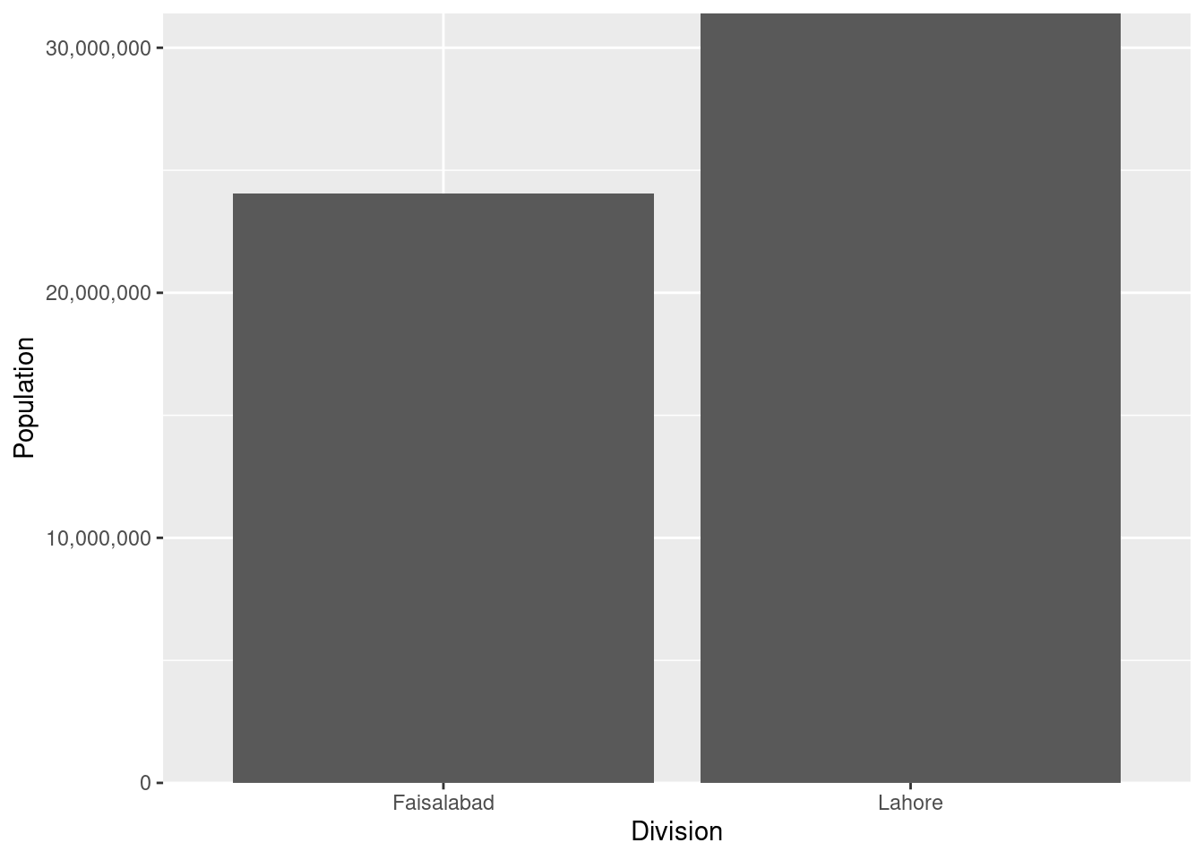
1 Punjab   Faisalabad Pop2017   14177081
2 Punjab   Lahore     Pop2017   19398081
3 Punjab   Faisalabad Pop1998    9885685
4 Punjab   Lahore     Pop1998   12015649

g<-ggplot(data = plotUnit, mapping = aes(x = Division, y = Population))
g

g<-ggplot(data = plotUnit, mapping = aes(x = Division, y = Population))+
  geom_col()
g

g<-ggplot(data = plotUnit, mapping = aes(x = Division, y = Population))+
  geom_col()+
  scale_y_continuous(labels= scales::comma, expand =  c(0, 0))
g

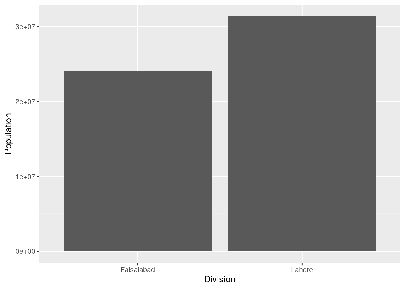
g<-ggplot(data = plotUnit, mapping = aes(x = Division, y = Population))+
  geom_bar(stat = "identity", position = position_dodge(width = .9))+
  scale_y_continuous(labels= scales::comma, expand =  c(0, 0))
g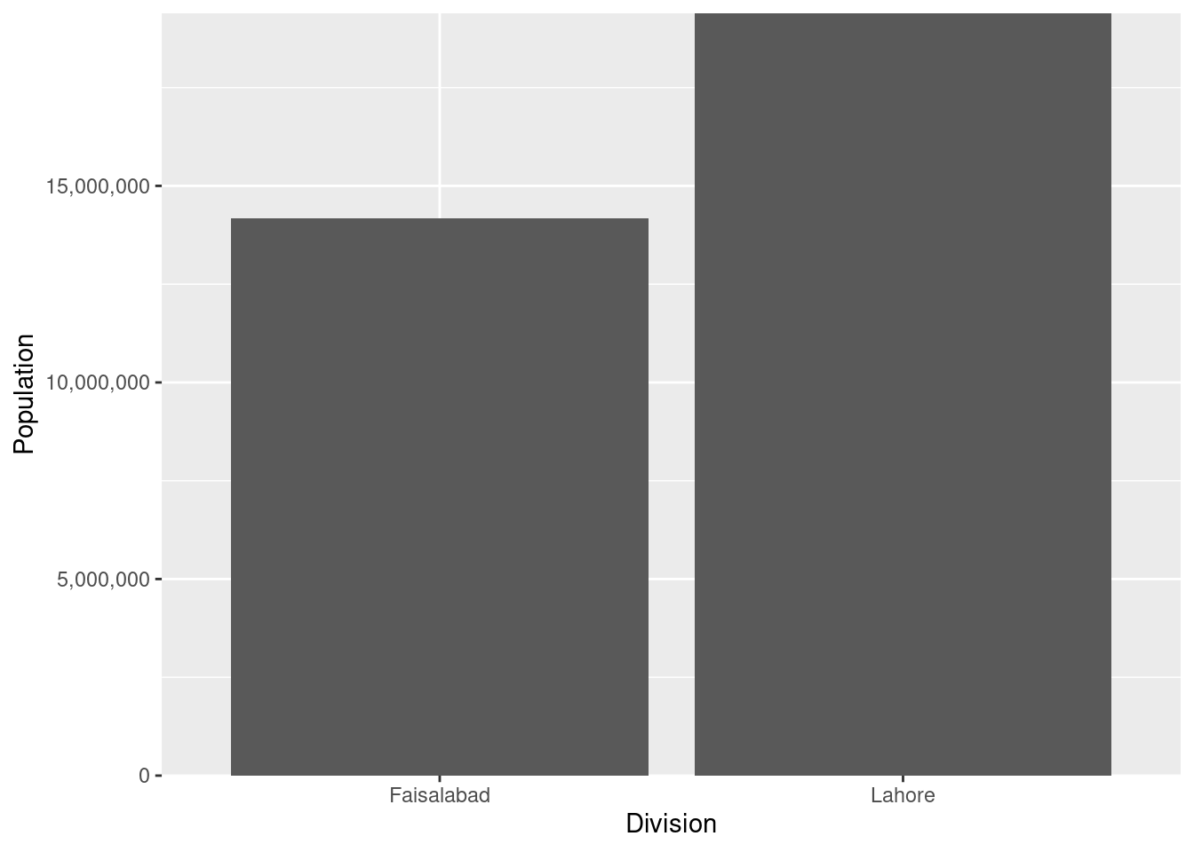

g<-ggplot(data = plotUnit,
          mapping = aes(x = Division, y = Population, fill = Census))+
  geom_bar(stat = "identity", position = position_dodge(width = .9))+
  scale_y_continuous(labels= scales::comma, expand =  c(0, 0))
g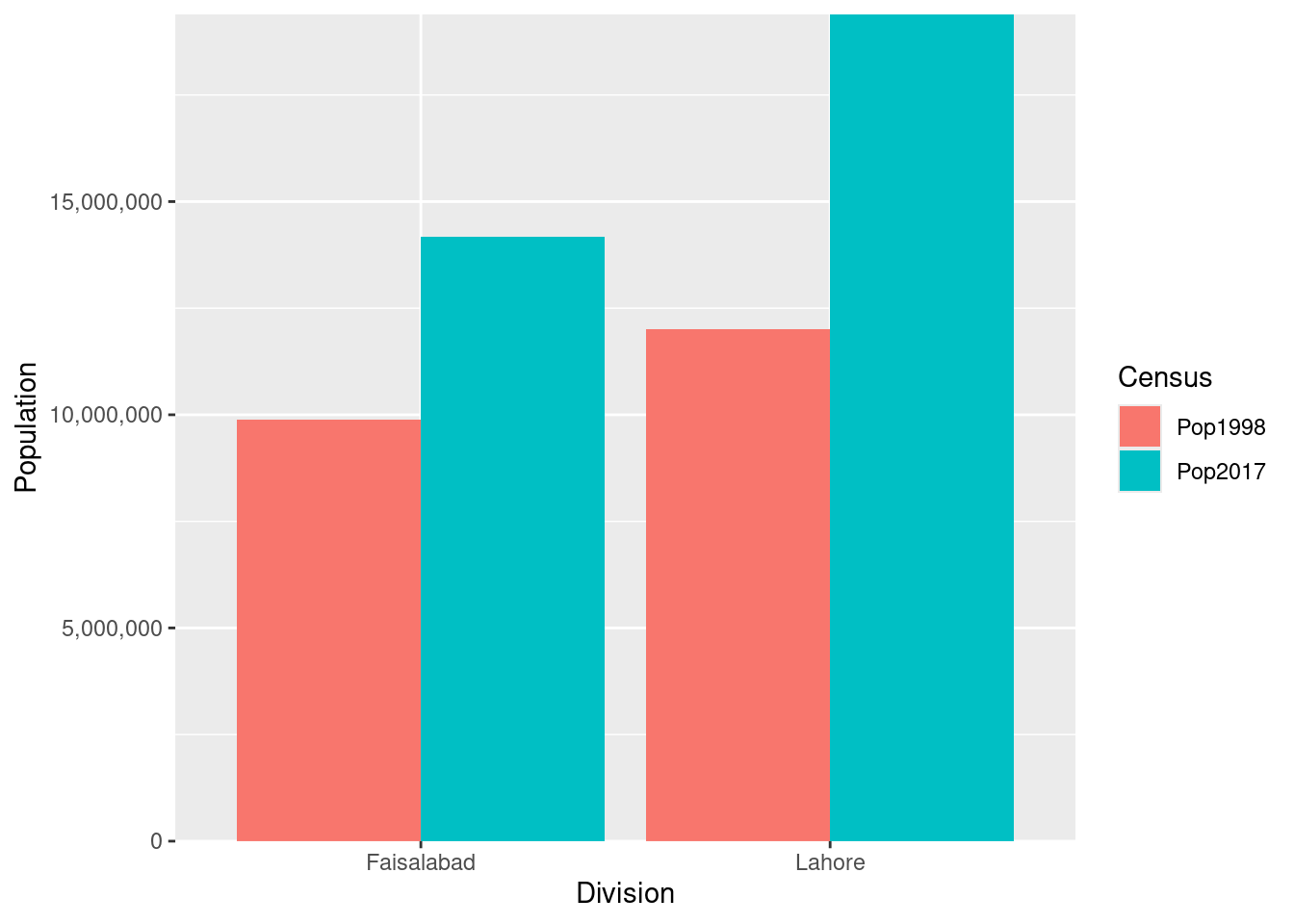

g<-ggplot(data = plotUnit,
          mapping = aes(x = Division, y = Population, fill = Census))+
  geom_bar(stat = "identity", position = position_dodge(width = .9))+
  scale_y_continuous(labels= scales::comma, expand =  c(0, 0))+
  geom_text(aes(label=scales::comma(Population)),
            position=position_dodge(width = 0.9), vjust = 0.8)
g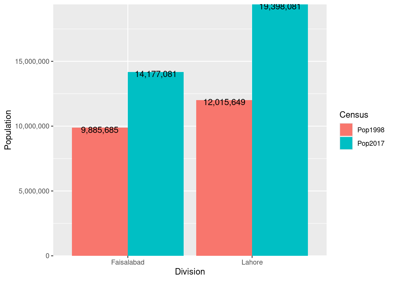

g<-ggplot(data = plotUnit,
          mapping = aes(x = Division, y = Population, fill = Census))+
  geom_bar(stat = "identity", position = position_dodge(width = .9))+
  scale_y_continuous(labels= scales::comma, expand =  c(0, 0))+
  geom_text(aes(label=scales::comma(Population)),
            position=position_dodge(width = 0.9), vjust = 0.8)+
  facet_wrap(~Province, scales = "free_x")
g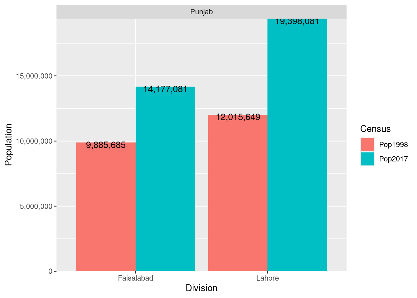

plotUnit <-
  PakPC2017Tehsil %>%
  dplyr::group_by(Province, Division) %>%
  dplyr::summarize(
    Pop2017 = sum(Pop2017, na.rm = TRUE)
    , Pop1998 = sum(Pop1998, na.rm = TRUE)
  ) %>%
  dplyr::filter(Division %in% c("Faisalabad","Lahore", "Karachi", "Quetta")) %>%
  tidyr::gather(
    key   = "Census"
    , value = "Population"
    , -Province, - Division
  )

g<-ggplot(data = plotUnit,
          mapping = aes(x = Division, y = Population, fill = Census))+
  geom_bar(stat = "identity", position = position_dodge(width = .9))+
  scale_y_continuous(labels= scales::comma, expand =  c(0, 0))+
  geom_text(aes(label=scales::comma(Population)),
            position=position_dodge(width = 0.9), vjust = 0.8)+
  facet_wrap(~Province, scales = "free_x")
g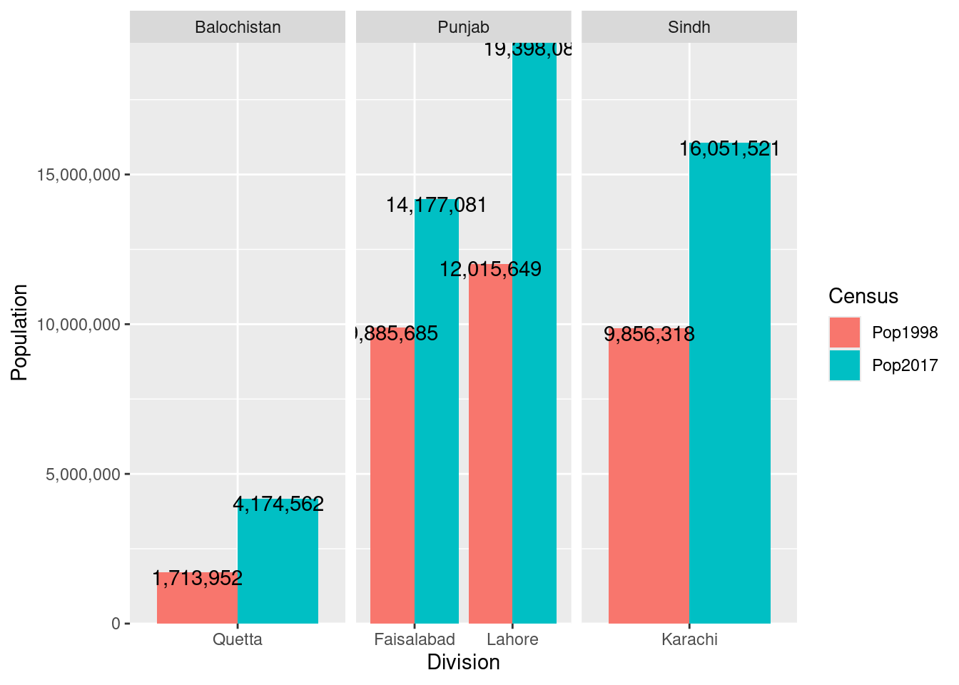

g<-ggplot(data = PakPC2017Pakistan, mapping = aes(x = Province, y = Pop2017))
g+geom_point(aes(color = ResStatus))+theme(legend.position = "top")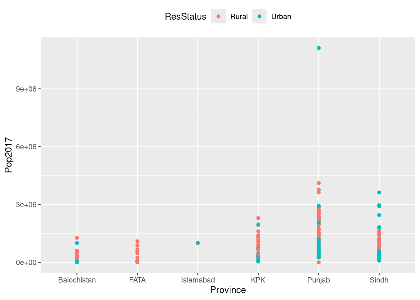

Scatter Plot

ggplot(PakPC2017Tehsil, aes(Pop1998,Pop2017))+geom_point()+geom_smooth(method = lm)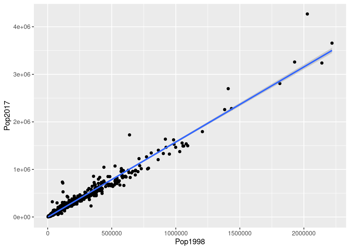

dygraphs

The dygraphs package is an R interface to the dygraphs JavaScript charting library. It provides rich facilities for charting time-series data in R

library(dygraphs)
dygraph(nhtemp, main = "New Haven Temperatures", ylab = "Temp (F)")

lungDeaths <- cbind(mdeaths, fdeaths)
dygraph(lungDeaths)

dygraph(lungDeaths) %>% dyRangeSelector()

dygraph(lungDeaths) %>%
  dySeries("mdeaths", label = "Male") %>%
  dySeries("fdeaths", label = "Female") %>%
  dyOptions(stackedGraph = TRUE) %>%
  dyRangeSelector(height = 10)

Year<-seq(from = as.Date("1990/1/1"), to = as.Date("2018/1/1"), by = "years")
prod<-rnorm(29,0,1)
timeSeries<-xts::xts(prod,Year)
dygraph(timeSeries)

plotly

library(ggplot2)
library(plotly)
myPlot<-ggplot(data = mpg, mapping = aes(x = displ, y = hwy))+
  geom_point(mapping = aes(color = drv))+
  geom_smooth(mapping = aes(linetype = drv))
ggplotly(myPlot)

datatable

library(readxl)
spi <- read_excel("C:/Users/PBS FAISALABAD/Desktop/spi.xls")
DT::datatable(spi,fillContainer = TRUE, editable = TRUE)

Citation

BibTeX citation:

@online{arfan_dilber2018,
  author = {Arfan Dilber, Muhammad},
  title = {Data {Analysis} with {R:} {Introduction} of {R} {Language}},
  date = {2018-03-25},
  url = {https://myaseen208.com/blogs/2018-03-25_Maldives_R/},
  langid = {en}
}

For attribution, please cite this work as:

Arfan Dilber, Muhammad. 2018. “Data Analysis with R: Introduction of R Language.” March 25, 2018. https://myaseen208.com/blogs/2018-03-25_Maldives_R/.